Solving Problems Submitted to MAA Journals (Part 5a)

The following problem appeared in Volume 96, Issue 3 (2023) of Mathematics Magazine.

Evaluate the following sums in closed form:

$\displaystyle \sum_{n=0}^\infty \left( \cos x - 1 + \frac{x^2}{2!} - \frac{x^4}{4!} \dots + (-1)^{n-1} \frac{x^{2n}}{(2n)!} \right)$

and

$\displaystyle \sum_{n=0}^\infty \left( \sin x - x + \frac{x^3}{3!} - \frac{x^5}{5!} \dots + (-1)^{n-1} \frac{x^{2n+1}}{(2n+1)!} \right)$ .

When I first read this problem, I immediately noticed that

$\displaystyle 1 - \frac{x^2}{2!} + \frac{x^4}{4!} \dots - (-1)^{n-1} \frac{x^{2n}}{(2n)!} \right)$

is a Taylor polynomial of $\cos x$ and

$\displaystyle x - \frac{x^3}{3!} + \frac{x^5}{5!} \dots - (-1)^{n-1} \frac{x^{2n+1}}{(2n+1)!} \right)$

is a Taylor polynomial of $\sin x$ . In other words, the given expressions are the sums of the tail-sums of the Taylor series for $\cos x$ and $\sin x$ .

As usual when stumped, I used technology to guide me. Here’s the graph of the first sum, adding the first 50 terms.

I immediately notice that the function oscillates, which makes me suspect that the answer involves either $\cos x$ or $\sin x$ . I also notice that the sizes of oscillations increase as $|x|$ increases, so that the answer should have the form $g(x) \cos x$ or $g(x) \sin x$ , where $g$ is an increasing function. I also notice that the graph is symmetric about the origin, so that the function is even. I also notice that the graph passes through the origin.

So, taking all of that in, one of my first guesses was $y = x \sin x$ , which is satisfies all of the above criteria.

That’s not it, but it’s not far off. The oscillations of my guess in orange are too big and they’re inverted from the actual graph in blue. After some guessing, I eventually landed on $y = -\frac{1}{2} x \sin x$ .

That was a very good sign… the two graphs were pretty much on top of each other. That’s not a proof that $-\frac{1}{2} x \sin x$ is the answer, of course, but it’s certainly a good indicator.

I didn’t have the same luck with the other sum; I could graph it but wasn’t able to just guess what the curve could be.

Solving Problems Submitted to MAA Journals (Part 4)

The following problem appeared in Volume 96, Issue 3 (2023) of Mathematics Magazine.

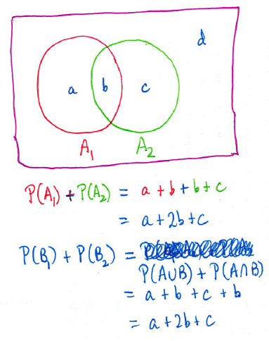
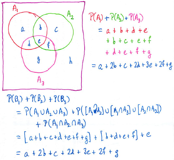
Let $A_1, \dots, A_n$ be arbitrary events in a probability field. Denote by $B_k$ the event that at least $k$ of $A_1, \dots A_n$ occur. Prove that $\displaystyle \sum_{k=1}^n P(B_k) = \sum_{k=1}^n P(A_k)$ .

I’ll admit when I first read this problem, I didn’t believe it. I had to draw a couple of Venn diagrams to convince myself that it actually worked:

Of course, pictures are not proofs, so I started giving the problem more thought.

I wish I could say where I got the inspiration from, but I got the idea to define a new random variable $N$ to be the number of events from $A_1, \dots A_n$ that occur. With this definition, $B_k$ becomes the event that $N \ge k$ , so that

$\displaystyle \sum_{k=1}^n P(B_k) = \sum_{k=1}^n P(N \ge k)$

At this point, my Spidey Sense went off: that’s the tail-sum formula for expectation! Since $N$ is a non-negative integer-valued random variable, the mean of $N$ can be computed by

$E(N) = \displaystyle \sum_{k=1}^n P(N \ge k)$ .

Said another way, $E(N) = \displaystyle \sum_{k=1}^n P(B_k)$ .

Therefore, to solve the problem, it remains to show that $\displaystyle \sum_{k=1}^n P(A_k)$ is also equal to $E(N)$ . To do this, I employed the standard technique from the bag of tricks of writing $N$ as the sum of indicator random variables. Define

$I_k = \displaystyle \bigg\{ \begin{array}{ll} 1, & A_k \hbox{~occurs} \\ 0, & A_k \hbox{~does not occur} \end{array}$

Then $N = I_1 + \dots + I_n$ , so that

$E(N) = \displaystyle \sum_{k=1}^n E(I_k) =\sum_{k=1}^n [1 \cdot P(A_k) + 0 \cdot P(A_k^c)] =\sum_{k=1}^n P(A_k)$ .

Equating the two expressions for $E(N)$ , we conclude that $\displaystyle \sum_{k=1}^n P(B_k) = \sum_{k=1}^n P(A_k)$ , as claimed.

Solving Problems Submitted to MAA Journals (Part 3)

The following problem appeared in Volume 53, Issue 4 (2022) of The College Mathematics Journal.

Define, for every non-negative integer $n$ , the $n$ th Catalan number by

$C_n := \displaystyle \frac{1}{n+1} {2n \choose n}$ .

Consider the sequence of complex polynomials in $z$ defined by $z_k := z_{k-1}^2 + z$ for every non-negative integer $k$ , where $z_0 := z$ . It is clear that $z_k$ has degree $2^k$ and thus has the representation

$z_k =\displaystyle \sum_{n=1}^{2^k} M_{n,k} z^n$ ,

where each $M_{n,k}$ is a positive integer. Prove that $M_{n,k} = C_{n-1}$ for $1 \le n \le k+1$ .

This problem appeared in the same issue as the probability problem considered in the previous two posts. Looking back, I think that the confidence that I gained by solving that problem gave me the persistence to solve this problem as well.

My first thought when reading this problem was something like “This involves sums, polynomials, and binomial coefficients. And since the sequence is recursively defined, it’s probably going to involve a proof by mathematical induction. I can do this.”

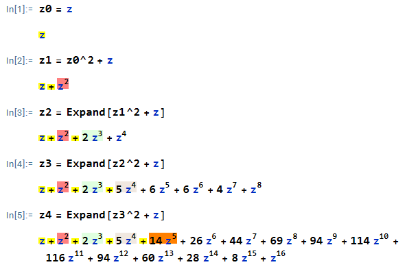
My second thought was to use Mathematica to develop my own intuition and to confirm that the claimed pattern actually worked for the first few values of $z_k$ .

As claimed in the statement of the problem, each $z_k$ is a polynomial of degree $2^k$ without a nontrivial constant term. Also, for each $z_k$ , the term of degree $n$ , for $1 \le n \le k+1$ , has a coefficient that is independent of $k$ which equal to $C_{n-1}$ . For example, for $z_4$ , the coefficient of $z^5$ (in orange above) is equal to

$C_4 = \displaystyle \frac{1}{5} {8 \choose 4} = \frac{8!}{4! 4! \cdot 5} = \frac{40320}{2880} = 14$ ,

and the problem claims that the coefficient of $z^5$ will remain 14 for $z_5, z_6, z_7, \dots$

Confident that the pattern actually worked, all that remained was pushing through the proof by induction.

We proceed by induction on $k$ . The statement clearly holds for $k=1$ :

$z_1 = z_0^2 + z = z + z^2 = C_0 z + C_1 z^2$ .

Although not necessary, I’ll add for good measure that

$z_2 = z_1^2 + z = (z^2+z)^2 + z = z + z^2 + 2z^3 + z^4 = C_0 z + C_1 z^2 + C_2 z^3 + z^4$

and

$z_3 = z^2 + z = (z^4+2z^3+z^2+z)^2 + z$

$= z + z^2 + 2z^3 + 5z^4 + 6z^5 + 6z^6 + 4z^7 + z^8$

$= C_0 z + C_1 z^2 + C_2 z^3 + C_3 z^4 + 6z^5 + 6z^6 + 4z^7 + z^8.$

This next calculation illustrates what’s coming later. In the previous calculation, the coefficient of $z^4$ is found by multiplying out

$(z^4+2z^3+z^2+z)(z^4+2z^3+z^2+z)$ .

This is accomplished by examining all pairs, one from the left product and one from the right product, so that the exponent works out to be $z^4$ . In this case, it’s

$(2z^3)(z) + (z^2)(z^2) + (z)(2z^3) = 5z^4$ .

For the inductive step, we assume that, for some $k \ge 1$ , $M_{n,k} = C_{n-1}$ for all $1 \le n \le k+1$ , and we define

$z_{k+1} = z + \left( M_{1,k} z + M_{2,k} z^2 + M_{3,k} z^3 + \dots + M_{2^k,k} z^{2^k} \right)^2$

Our goal is to show that $M_{n,k+1} = C_{n-1}$ for $n = 1, 2, \dots, k+2$ .

For $n=1$ , the coefficient $M_{1,k+1}$ of $z$ in $z_{k+1}$ is clearly 1, or $C_0$ .

For $2 \le n \le k+2$ , the coefficient $M_{n,k+1}$ of $z^n$ in $z_{k+1}$ can be found by expanding the above square. Every product of the form $M_{j,k} z^j \cdot M_{n-j,k} z^{n-j}$ will contribute to the term $M_{n,k+1} z^n$ . Since $n \le k+2 \le 2^k+1$ (since $k \ge 1$ ), the values of $j$ that will contribute to this term will be $j = 1, 2, \dots, n-1$ . (Ordinarily, the $z^0$ and $z^n$ terms would also contribute; however, there is no $z^0$ term in the expression being squared). Therefore, after using the induction hypothesis and reindexing, we find

$M_{n,k+1} = \displaystyle \sum_{j=1}^{n-1} M_{j,k} M_{n-j,k}$

$= \displaystyle\sum_{j=1}^{n-1} C_{j-1} C_{n-j-1}$

$= \displaystyle\sum_{j=0}^{n-2} C_j C_{n-2-j}$

$= C_{n-1}$ .

The last step used a recursive relationship for the Catalan numbers that I vaguely recalled but absolutely had to look up to complete the proof.

Solving Problems Submitted to MAA Journals (Part 2b)

The following problem appeared in Volume 53, Issue 4 (2022) of The College Mathematics Journal. This was the second-half of a two-part problem.

Suppose that $X$ and $Y$ are independent, uniform random variables over $[0,1]$ . Define $U_X$ , $V_X$ , $B_X$ , and $W_X$ as follows:

$U_X$ is uniform over $[0,X]$ ,

$V_X$ is uniform over $[X,1]$ ,

$B_X \in \{0,1\}$ with $P(B_X=1) = X$ and $P(B_X=0)=1-X$ , and

$W_X = B_X \cdot U_X + (1-B_X) \cdot V_X$ .

Prove that $W_X$ is uniform over $[0,1]$ .

Once again, one way of showing that $W_X$ is uniform on $[0,1]$ is showing that $P(W_X \le t) = t$ if $0 \le t \le 1$ .

My first thought was that the value of $W_X$ depends on the value of $X$ , and so it makes sense to write $P(W_X \le t)$ as an integral of conditional probabilities:

$P(W_X \le t) = \displaystyle \int_0^1 P(W_X \le t \mid X = x) f(x) \, dx$ ,

where $f(x)$ is the probability density function of $X$ . In this case, since $X$ has a uniform distribution over $[0,1]$ , we see that $f(x) = 1$ for $0 \le x \le 1$ . Therefore,

$P(W_X \le t) = \displaystyle \int_0^1 P(W_X \le t \mid X = x) \, dx$ .

My second thought was that $W_X$ really has a two-part definition:

$W_X = \displaystyle \bigg\{ \begin{array}{ll} U_X, & B_X = 1 \\ V_X, & B_X = 0 \end{array}$

So it made sense to divide the conditional probability into these two cases:

$P(W_X \le t) = \displaystyle \int_0^1 P(W_X \le t, B_X = 1 ~\hbox{or}~ B_X = 0 \mid X = x) \, dx$

$= \displaystyle \int_0^1 P(W_X \le t, B_X = 1 \mid X = x) \, dx + \int_0^1 P(W_X \le t, B_X = 0 \mid X = x) \, dx$

My third thought was that these probabilities can be rewritten using the Multiplication Rule. This ordinarily has the form $P(E \cap F) = P(E) P(F \mid E)$ . For an initial conditional probability, it has the form $P(E \cap F \mid G) = P(E \mid G) P(F \mid E \cap G)$ . Therefore,

$P(W_X \le t) = \displaystyle \int_0^1 P(B_X = 1 \mid X = x) P(W_X \le t \mid B_X = 1, X = x) \, dx$

$+ \displaystyle \int_0^1 P(B_X = 0 \mid X=x) P(W_X \le t \mid B_X = 0, X = x) \, dx$ .

The definition of $B_X$ provides the immediate computation of $P(B_X = 1 \mid X = x)$ and $P(B_X = 0 \mid X = x)$ :

$P(W_X \le t) =\displaystyle \int_0^1 x P(W_X \le t \mid B_X = 1, X = x) \, dx$

$+ \displaystyle \int_0^1 (1-x) P(W_X \le t \mid B_X = 0, X = x) \, dx$

Also, the two-part definition of $W_X$ provides the next step:

$P(W_X \le t) =\displaystyle \int_0^1 x P(U_X \le t \mid B_X = 1, X = x) \, dx$

$+ \displaystyle \int_0^1 (1-x) P(V_X \le t \mid B_X = 0, X = x) \, dx$

We split each of these integrals into an integral from $0$ to $t$ and then an integral from $t$ to $1$ . First,

$\displaystyle \int_0^1 x P(U_X \le t \mid B_X = 1, X = x) \, dx$

$= \displaystyle \int_0^t x P(U_X \le t \mid B_X = 1, X = x) \, dx + \displaystyle \int_t^1 x P(U_X \le t \mid B_X = 1, X = x) \, dx$ .

We now use the following: if $0 \le x \le 1$ and $U$ is uniform over $[0,x]$ , then

$P(U \le t) = \displaystyle \bigg\{ \begin{array}{ll} t/x, & t \le x \\ 1, & t > x \end{array}$

We observe that $t > x$ in the first integral, while $t \le x$ in the second integral. Therefore,

$\displaystyle \int_0^1 x P(U_X \le t \mid B_X = 1, X = x) \, dx = \int_0^t x \cdot 1 \, dx + \int_t^1 x \cdot \frac{t}{x} \, dx$

$= \displaystyle \int_0^t x \, dx + \int_t^1 t \, dx$ .

For the second integral involving $V_X$ , we again split into two subintegrals and use the fact that if $V$ is uniform on $[x,1]$ , then

$P(V \le t) = \displaystyle \bigg\{ \begin{array}{ll} 0, & t \le x \\ (t-x)/(1-x), & t > x \end{array}$

Therefore,

$\displaystyle \int_0^1 (1-x) P(V_X \le t \mid B_X = 0, X = x) \, dx$

$=\displaystyle \int_0^t (1-x) P(V_X \le t \mid B_X = 0, X = x) \, dx$

$+ \displaystyle \int_t^1 (1-x) P(V_X \le t \mid B_X = 0, X = x) \, dx$

$= \displaystyle \int_0^t (1-x) \cdot \frac{t-x}{1-x} \, dx + \int_t^1 (1-x) \cdot 0 \, dx$

$= \displaystyle \int_0^t (t-x) \, dx$ .

Combining, we conclude that

$P(W_X \le t) = \displaystyle \int_0^t x \, dx + \int_t^1 t \, dx + \displaystyle \int_0^t (t-x) \, dx$

$= \displaystyle \int_0^t [x + (t-x)] \, dx + \int_t^1 t \, dx$

$= \displaystyle \int_0^t t \, dx + \int_t^1 t \, dx$

$= \displaystyle \int_0^1 t \, dx$

$= t$ ,

from which we conclude that $W_X$ is uniformly distributed on $[0,1]$ .

As I recall, this took a couple days of staring and false starts before I was finally able to get the solution.

Solving Problems Submitted to MAA Journals (Part 2a)

The following problem appeared in Volume 53, Issue 4 (2022) of The College Mathematics Journal. This was the first problem that was I able to solve in over 30 years of subscribing to MAA journals.

Suppose that $X$ and $Y$ are independent, uniform random variables over $[0,1]$ . Now define the random variable $Z$ by

$Z = (Y-X) {\bf 1}(Y \ge X) + (1-X+Y) {\bf 1}(Y<X)$ .

Prove that $Z$ is uniform over $[0,1]$ . Here, ${\bf 1}[S]$ is the indicator function that is equal to 1 if $S$ is true and 0 otherwise.

The first thing that went through my mind was something like, “This looks odd. But it’s a probability problem using concepts from a senior-level but undergraduate probability course. This was once my field of specialization. I had better be able to get this.”

My second thought was that one way of proving that $Z$ is uniform on $[0,1]$ is showing that $P(Z \le t) = t$ if $0 \le t \le 1$ .

My third thought was that $Z$ really had a two-part definition:

$Z = \bigg\{ \begin{array}{ll} Y-X, & Y \ge X \\ 1-X+Y, & Y <X \end{array}$

So I got started by dividing this probability into the two cases:

$P(Z \le t) = P(Z \le t, Y \ge X ~\hbox{or}~ Y < X)$

$= P(Z \le t, Y \ge X ~\hbox{or}~ Z \le t, Y < X)$

$= P(Z \le t, Y \ge X) + P(Z \le t, Y < X)$

$= P(Y-X \le t, Y \ge X) + P(1 - X + Y \le t, Y < X)$

$= P(Y \le X + t, Y \ge X) + P( Y \le X + t - 1, Y < X)$

$= P(X \le Y \le X + t) + P(Y \le X + t - 1)$ .

In the last step, since $0 \le t \le 1$ , the events $Y \le X + t - 1$ and $Y < X$ are redundant: if $Y \le X + t - 1$ , then $Y$ will automatically be less than $X$ . Therefore, it’s safe to remove $Y < X$ from the last probability.

Ordinarily, such probabilities are computed by double integrals over the joint probability density function of $X$ and $Y$ , which usually isn’t easy. However, in this case, since $X$ and $Y$ are independent and uniform over $[0,1]$ , the ordered pair $(X,Y)$ is uniform on the unit square $[0,1] \times [0,1]$ . Therefore, probabilities can be found by simply computing areas.

In this case, since the area of the unit square is 1, $P(Z \le t)$ is equal to the sum of the areas of

$\{(x,y) \in [0,1] \times [0,1] : x \le y \le x + t \}$ ,

which is depicted in green below, and

$\{(x,y) \in [0,1] \times [0,1] : y \le x + t - 1 \}$ ,

which is depicted in purple.

First, the area in green is a trapezoid. The $y-$ intercept of the line $y = x+t$ is $(0,t)$ , and the two lengths of $t$ and $1-t$ on the upper left of the square are found from this $y-$ intercept. The area of the green trapezoid is easiest found by subtracting the areas of two isosceles right triangles:

$latex \displaystyle \frac{(1)^2}{2} – \frac{(1-t)^2}{2} = \frac{1-1+2t-t^2}{2} = \frac{2t-t^2}{2}.

Second, the area in purple is an isosceles right triangle. The $y-$ intercept of the line $y=x+t-1$ is $(0,t-1)$ , so that the distance from the $y-$ intercept to the origin is $1-t$ . From this, the two lengths of $1-t$ and $t$ are found. Therefore, the area of the purple right triangle is $\displaystyle \frac{t^2}{2}$ .

Adding, we conclude that

$P(Z \le t) = \displaystyle \frac{2t-t^2}{2} + \frac{t^2}{2} = \frac{2t}{2} = t$ .

Therefore, $Z$ is uniform over $[0,1]$ .

A closing note: after going 0-for-4000 in my previous 30+ years of attempting problems submitted to MAA journals, I was unbelievably excited to finally get one. As I recall, it took me less than an hour to get the above solution, although writing up the solution cleanly took longer.

However, the above was only Part 1 of a two-part problem, so I knew I just had to get the second part before submitting. That’ll be the subject of the next post.

Solving Problems Submitted to MAA Journals (Part 1)

I first became a member of the Mathematical Association of America in 1988. My mentor in high school gave me a one-year membership as a high school graduation present, and I’ve maintained my membership ever since. Most years, I’ve been a subscriber to three journals: The American Mathematical Monthly, Mathematics Magazine, and College Mathematics Journal.

A feature for each of these journals is the Problems/Solutions section. In a nutshell, readers devise and submit original problems in mathematics for other readers to solve; the editors usually allow readers to submit solutions for a few months after the problems are first published. Between the three journals, something like 120 problems are submitted annually by readers.

And, historically, I had absolutely no success in solving these problems. Said another way: over my first 30+ years as an MAA member, I went something like 0-for-4000 at solving these submitted problems. This gnawed at me for years, especially when I read the solutions offered by other readers, maybe a year after the problem originally appeared, and thought to myself, “Why didn’t I think of that?”

Well, to be perfectly honest, that’s still my usual. However, in the past couple of years, I actually managed to solve a handful of problems that appeared in Mathematics Magazine and College Mathematics Journal, to my great surprise and delight. I don’t know what happened. Maybe I’ve just got better at problem solving. Maybe solving the first one or two boosted my confidence. Maybe success breeds success. Maybe all the hard problems have already been printed and the journals’ editors have nothing left to publish except relatively easier problems.

In this short series, I’ll try to reconstruct my thought processes and flashes of inspiration that led to these solutions.

500,000 page views

I’m taking a break from my usual posts on mathematics and mathematics education to note a symbolic milestone: meangreenmath.com has had more than 500,000 total page views since its inception in June 2013. Many thanks to the followers of this blog, and I hope that you’ll continue to find this blog to be a useful resource to you.

Thirty most viewed individual posts:

Thirty most viewed series:

2048 and algebra
Another poorly written word problem
Area of a triangle and volume of common shapes
Arithmetic and geometric series
Calculators and complex numbers
Common Core, subtraction, and the open number line
Computing e to any power
Confirming Einstein’s theory of general relativity with calculus
Day One of my Calculus I class
Different definitions of e
Exponential growth and decay
Facebook birthday problem
Fun lecture on geometric series
How I impressed my wife: $\displaystyle \int_0^{2\pi} \frac{dx}{\cos^2 x + 2 a \sin x \cos x + (a^2 + b^2) \sin^2 x}$
Inverse Functions
Langley’s Adventitious Angles
Lessons from teaching gifted elementary students
My favorite one-liners
My mathematical magic show
Parabolas from string art
Predicate logic and popular culture
Proving theorems and special cases
Reminding students about Taylor series
Slightly incorrect ugly mathematical Christmas T-shirts
Square roots and logarithms without a calculator
The antiderivative of $\displaystyle \frac{1}{x^4+1}$
Thoughts on 1/7 and other rational numbers
Thoughts on numerical integration
Wason selection task
Why does $x^0 = 1$ and $x^{-n} = 1/x^n$ ?

Thirty most viewed posts (guest presenters):

If I’m still here at that time, I’ll make a summary post like this again when this blog has over 1,000,000 page views.

My Favorite One-Liners: Index

I’m doing something that I should have done a long time ago: collecting a series of posts into one single post. The links below show my series on my favorite one-liners.

Mathematical Wisecracks for Almost Any Occasion: Part 2, Part 7, Part 8, Part 12, Part 21, Part 28, Part 29, Part 41, Part 46, Part 53, Part 60, Part 63, Part 65, Part 71, Part 79, Part 84, Part 85, Part 100, Part 101, Part 108, Part 109, Part 114, Part 118, Part 121

All-Purpose Anecdotes: Part 38, Part 50, Part 64, Part 70, Part 92, Part 94

Addressing Misconceptions: Part 3, Part 4, Part 11, Part 14, Part 15, Part 18, Part 30, Part 32, Part 33, Part 37, Part 45, Part 59

Tricky Steps in a Calculation: Part 5, Part 6

Greek alphabet and choice of variables: Part 40, Part 43, Part 56

Homework and exams: Part 39, Part 47, Part 55, Part 57, Part 58, Part 66, Part 77, Part 78, Part 91, Part 96, Part 97, Part 107

Inequalities: Part 99

Simplification: Part 10, Part 102, Part 103

Polynomials: Part 19, Part 48, Part 49, Part 81, Part 90

Inverses: Part 16

Exponential and Logarithmic Functions: Part 1, Part 42, Part 68, Part 80, Part 110

Trigonometry: Part 9, Part 69, Part 76, Part 106, Part 120

Complex numbers: Part 54, Part 67, Part 86, Part 112, Part 113

Sequences and Series: Part 20, Part 35, Part 111

Combinatorics: Part 27

Statistics: Part 22, Part 23, Part 36, Part 51, Part 52, Part 61, Part 95, Part 116

Probability: Part 26, Part 31, Part 62, Part 93, Part 122

Calculus: Part 24, Part 25, Part 72, Part 73, Part 74, Part 75, Part 83, Part 87, Part 88, Part 104, Part 115, Part 117

Logic and Proofs: Part 13, Part 17, Part 34, Part 44, Part 89, Part 98, Part 119

Differential Equations: Part 82, Part 105

Confirming Einstein’s General Theory of Relativity with Calculus: Index

I’m doing something that I should have done a long time ago: collecting a series of posts into one single post. The links below show my series on general relativity and the precession of Mercury’s orbit.

Part 1: Introduction

Part 1a: Introduction
Part 1b: Observed precession of Mercury
Part 1c: Outline of argument

Part 2: Precession, polar coordinates, and conic sections

Part 2a: Graphically exploring precession
Part 2b: Polar coordinates and ellipses
Part 2c: Polar coordinates, circles, and parabolas
Part 2d: Polar coordinates and hyperbolas

Part 3: Method of successive approximations

Part 4: Principles from physics

Part 4a: Angular momentum
Part 4b: Acceleration in polar coordinates
Part 4c: Newton’s Second Law and Newton’s Law of Gravitation

Part 5: Orbits under Newtonian mechanics

Part 5a: Confirmation of solution
Part 5b: Derivation with calculus
Part 5c: Derivation with differential equations and the method of undetermined coefficients
Part 5d: Derivation with differential equations and variation of parameters

Part 6: Orbits under general relativity

Part 6a: New differential equation under general relativity
Part 6b: Confirmation of solution
Part 6c: Derivation with variation of parameters
Parts 6d, 6e, 6f, 6g, 6h, 6i, 6j: Rationale for the method of undetermined coefficients
Part 6k: Derivation with undetermined coefficients

Part 7: Computing precession

Parts 7a, 7b, 7c, 7d: Predicting precession
Part 7e: Computing precession

Part 8: Second- and third-order solutions with the method of successive approximations

Part 9: Pedagogical thoughts

Earlier this year, I presented these ideas for the UNT Math Department’s Undergraduate Mathematics Colloquium Series. The video of my lecture is below.

My Mathematical Magic Show: Index

I’m doing something that I should have done a long time ago: collecting a series of posts into one single post. The links below show the mathematical magic show that I’ll perform from time to time.

Part 1: Introduction.

Part 2a, Part 2b, and Part 2c: The 1089 trick.

Part 3a, Part 3b, and Part 3c: A geometric magic trick.

Part 4a: Part 4b, Part 4c, and Part 4d: A trick using binary numbers.

Part 5a, Part 5b, Part 5c, and Part 5d: A trick using the rule for checking if a number is a multiple of 9.

Part 7: The Fitch-Cheney card trick, which is perhaps the slickest mathematical card trick ever devised.

Part 8a, Part 8b, and Part 8c: A trick using Pascal’s triangle.

Part 9: Mentally computing $n$ given $n^5$ if $10 \le n \le 99$ .

Part 10: A mathematical optical illusion.

Part 11: The 27-card trick, which requires representing numbers in base 3.

Part 6: The Grand Finale.

And, for the sake of completeness, here’s a picture of me just before I performed an abbreviated version of this show for UNT’s Preview Day for high school students thinking about enrolling at my university.