I really liked xkcd’s take on numerical analysis and error propagation:
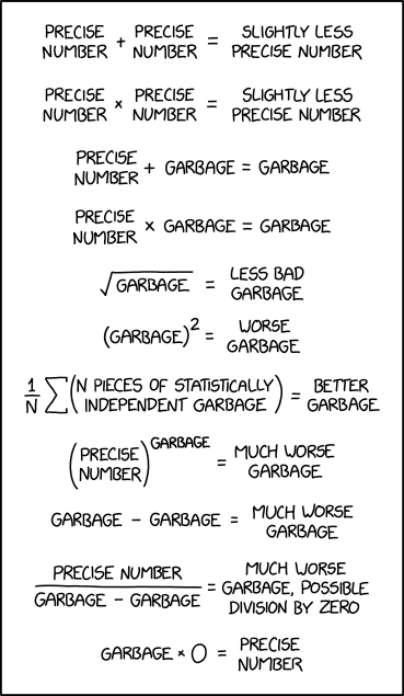
Source: https://xkcd.com/2295/
A good mathematical explanation of this comic can be found here: https://www.explainxkcd.com/wiki/index.php/2295:_Garbage_Math
I really liked xkcd’s take on numerical analysis and error propagation:
Source: https://xkcd.com/2295/
A good mathematical explanation of this comic can be found here: https://www.explainxkcd.com/wiki/index.php/2295:_Garbage_Math
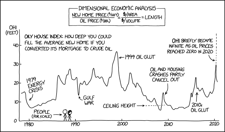
Source: https://xkcd.com/2327/
From the YouTube description:
Erica Flapan (Pomona College) explains why it is important to determine whether a molecule has mirror image symmetry, and discusses the differences between a geometric, chemical, and topological approach to understanding mirror image symmetry.
In this series of posts, I provide a deeper look at common applications of exponential functions that arise in an Algebra II or Precalculus class. In the previous posts in this series, I considered financial applications. In today’s post, I’ll discuss radioactive decay and the half-life formula.
One way of writing the formula for how a radioactive substance (carbon-14, uranium-235, brain cells) decays is
In yesterday’s post, I showed how this formula is a natural consequence of a certain differential equation. Of course, students in Algebra II or Precalculus (or high school chemistry) are usually not ready to understand this derivation using calculus. Instead, they are typically given the final formula and are expected to use this formula to solve problems. Still, I think it’s important for the teacher of Algebra II or Precalculus to be aware of how the origins of this formula, as it only requires mathematics that’s only a year or two away in these students’ mathematical development.
There is another correct way to write this formula in terms of half-life. Sadly, my experience is that many students are familiar with these two different formulas but are not aware of how the two formulas are connected. As we’ll see, while yesterday’s post using differential equations is inaccessible to Algebra II and Precalculus students, the derivation below is entirely elementary and can be understood by good students in these courses.
Let 
Substituting into the above formula, we find
Let’s now solve for the constant 
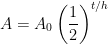
Let’s now substitute this back into the original formula:
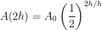
This is the usual half-life formula, where the previous base of 

In other words, after two half-life periods, only one-fourth (half of a half) of the substance remains.
In this series of posts, I provide a deeper look at common applications of exponential functions that arise in an Algebra II or Precalculus class. In the previous posts in this series, I considered financial applications. In today’s post, I’ll discuss radioactive decay and the half-life formula.
While these formulas are easy to state, not many high school teachers are aware of the physical principles from which they arise. The basic idea is that if amount 

The negative sign on the right-hand side isn’t strictly necessary, but it’s a reminder that amount present decreases as time increases.
This differential equation can be solved in several ways, including separation of variables (below, I’ll be sloppy with the constant of integration for the sake of simplicity):
To solve for the constant, we usually use the initial condition 
Plugging back in, we obtain the final answer
Of course, students in Algebra II or Precalculus (or high school chemistry) are usually not ready to understand this derivation using calculus. Instead, they are typically given the final formula and are expected to use this formula to solve problems. Still, I think it’s important for the teacher of Algebra II or Precalculus to be aware of how the origins of this formula, as it only requires mathematics that’s only a year or two away in these students’ mathematical development.
Shamelessly stolen from a friend:
How do you tell the difference between a plumber and a chemist?
Ask them to pronounce unionized.


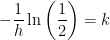

![A = A_0 e^{ -\left[ -\frac{1}{h} \ln \left( \frac{1}{2} \right) \right] t}](https://s0.wp.com/latex.php?latex=A+%3D+A_0+e%5E%7B+-%5Cleft%5B+-%5Cfrac%7B1%7D%7Bh%7D+%5Cln+%5Cleft%28+%5Cfrac%7B1%7D%7B2%7D+%5Cright%29+%5Cright%5D+t%7D&bg=ffffff&fg=000000&s=0&c=20201002)
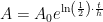
![A = A_0 \left[e^{\ln \left( \frac{1}{2} \right)} \right]^{t/h}](https://s0.wp.com/latex.php?latex=A+%3D+A_0+%5Cleft%5Be%5E%7B%5Cln+%5Cleft%28+%5Cfrac%7B1%7D%7B2%7D+%5Cright%29%7D+%5Cright%5D%5E%7Bt%2Fh%7D&bg=ffffff&fg=000000&s=0&c=20201002)