In my capstone class for future secondary math teachers, I ask my students to come up with ideas for engaging their students with different topics in the secondary mathematics curriculum. In other words, the point of the assignment was not to devise a full-blown lesson plan on this topic. Instead, I asked my students to think about three different ways of getting their students interested in the topic in the first place.
I plan to share some of the best of these ideas on this blog (after asking my students’ permission, of course).
This student submission comes from my former student Joe Wood. His topic, from Precalculus: inverse trigonometric functions.

What are the contributions of various cultures to this topic?
Trig functions have a very long history spanning many countries and cultures. Greek astronomers such as Aristarchus, Claudius, and Ptolemy first used trigonometry; however, according to the University of Connecticut, these Greek astronomers were primarily concerned with “the length of the chord of a circle as a function of the circular arc joining its endpoints.” Many of these astronomers, Ptolemy especially, were concerned with planetary and celestial body’s rotations, so this made sense.
While the Greeks first studied trigonometric concepts, it was the Indian people who really studied sine and cosine functions with the angle as a variable. The information was then brought to the Arabic and Persian cultures. One significant figure, a Persian by the name Abu Rayhan Biruni, used trig to accurately estimate the circumference of Earth and its radius before the end of the 11th century.
Fast-forward about 700 years, a Swiss mathematician, Daniel Bernoulli, used the “A.sin” notation to represent the inverse of sine. Shortly after, another Swiss mathematician used “A t” to represent the inverse of tangent. That man was none other than Leonhard Euler. It was not until 1813 that the notation sin-1 and tan-1 were introduced by Sir John Fredrick William Herschel, an English mathematician.
As we can see, the development of inverse trigonometric functions took quite the cultural rollercoaster ride before stopping some place we see being familiar. It took many cultures, and even more years to develop this sophisticated branch of mathematics.
How could you as a teacher create an activity or project that involves your topic?
Last Semester I taught a lesson on the trigonometric identities. I found this cool cut and paste activity for the students that allowed them to warm up to the trig identities by not having to do the process themselves, but still having to see every step of converting one trig function into another with the identities. Below, you will find the activity, then the instructions, and finally how to modify the activity to fit inverse trig identities specifically.

Directions:
1.) Begin by cutting out all the pieces.
2.) Students will take any of the four puzzle pieces with the black squiggly line.
3.) Find an equivalent puzzle piece by using some trig identity.
4.) Repeat step 3 until there are no more equivalent pieces.
5.) Grab the next puzzle pieces with the black squiggly line.
6.) Repeat steps 3-5 until all puzzle pieces have been used.
Ex.) Begin with cscx-sinx. Lay next to that piece, the piece that reads =1/sinx – sinx, then the piece that reads =1/sinx – sin2x/sinx. Contiue the trend until you reach =cotx * cosx. Then move to the next squiggly lined piece.
Modify:
This game can be modified using inverse trig functions. Start with pieces such as sin-1(sin(300)) in squiggles. Have a piece showing sin-1(sin(300)) with a line through the sines. Then a piece that just shows 300. Next a piece in a squiggly line that is sin-1(sqrt(2)/2) that connects to a piece of 450, but make them write why this works.
How does this topic extend what your students should have learned in previous courses?
Obviously, by this time students should know what trigonometric functions are and how to use this. Students should also know from previous classes what inverse functions are. Studying inverse trig functions then is a continuation of these topics. As I teacher I would begin relating inverse trig functions by refreshing the students on what inverse functions are. The class would then move into the concept that the trig expression of an angle returns a ratio of two sides of a triangle. We would slowly move into what happens then if you know the sides of a triangle but need the angle. From there we would discuss trigonometric expressions using the angles as variables. Finally, we would make the connection that that is a function, and on the proper interval should have an inverse function. That is when the extension into the new topic of inverse trigonometric functions would seriously begin.


 . I told the class that I had worked this out ahead of time, and that the approximate answer was
  . Then I used that angle for whatever I needed it for and continued until obtaining the eventual solution.
 ?
? , thanks to my calculation prior to class. I also knew that
  since the graph of
  has a vertical asymptote at
  . So the solution to
  had to be somewhere between
  .
. ,” I said, faking complete and utter confidence.
 .)
.)

 , and the substitution
  .
. .
. , the magic substitution

 and
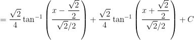
and  , there is an alternative answer:
 .
.
 .
. over an interval that contains neither
  or
or  , then either
  or
or  can be used. Courtesy of Mathematica:
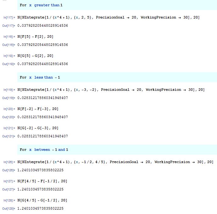
 (or both), then only using
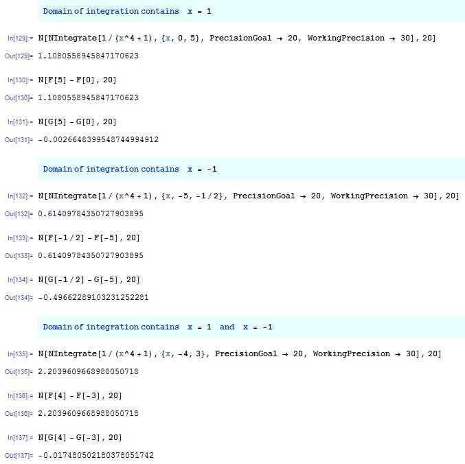
 that appeared several posts ago ultimately makes a big difference in the final answers that are obtained.
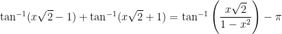 if
if  ,
, if
if  ,
, if
if  ,
, and
and  are the unique values so that
 ,
, .
. and
and  . Indeed, it’s apparent that these have to be the two transition points because these are the points where
  is undefined. However, it would be more convincing to show this directly.
 .
.
 and
and  , so that
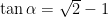 ,
, .
. and
and  can be represented in the figure below:
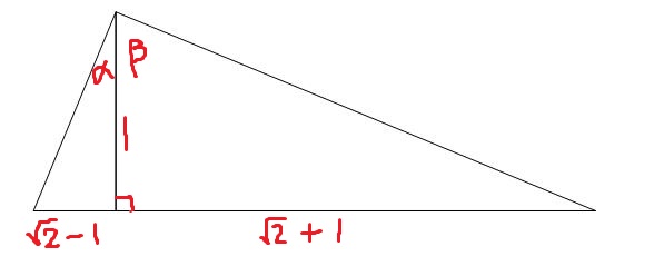
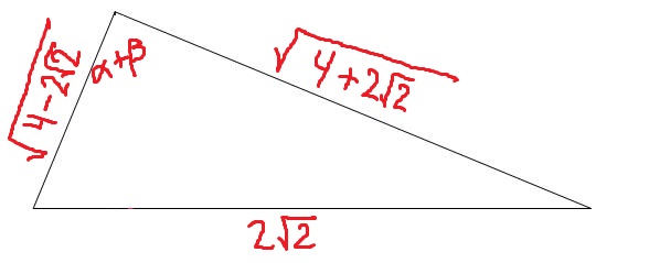
 . I will use the Pythagorean theorem to find the lengths of the other two sides. For the small right triangle containing

 ,
, .
. . In other words,
  is an odd function using the fact that
  is also an odd function:
![= \tan^{-1} ( -[x\sqrt{2} + 1] ) + \tan^{-1}( -[x \sqrt{2} - 1])](https://s0.wp.com/latex.php?latex=%3D+%5Ctan%5E%7B-1%7D+%28+-%5Bx%5Csqrt%7B2%7D+%2B+1%5D+%29+%2B+%5Ctan%5E%7B-1%7D%28+-%5Bx+%5Csqrt%7B2%7D+-+1%5D%29&bg=ffffff&fg=000000&s=0&c=20201002)

![= - \left[ \tan^{-1} ( x\sqrt{2} + 1 ) + \tan^{-1}( x \sqrt{2} - 1) \right]](https://s0.wp.com/latex.php?latex=%3D+-+%5Cleft%5B+%5Ctan%5E%7B-1%7D+%28+x%5Csqrt%7B2%7D+%2B+1+%29+%2B+%5Ctan%5E%7B-1%7D%28+x+%5Csqrt%7B2%7D+-+1%29+%5Cright%5D&bg=ffffff&fg=000000&s=0&c=20201002)
 .
. , and so
  ,
, ,
, .
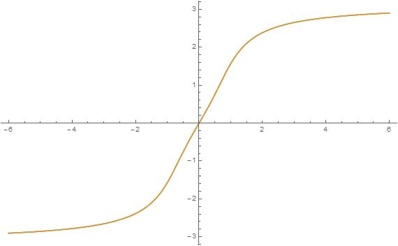
. and
and  are important. Without them, the graphs of the left-hand side and right-hand sides are clearly different if
  :
:
 and
and  , I know that
 ,
, ,
, .
. ,
, and
and  must differ if
  is in the interval
 ![[-\pi,-\pi/2]](https://s0.wp.com/latex.php?latex=%5B-%5Cpi%2C-%5Cpi%2F2%5D&bg=ffffff&fg=000000&s=0&c=20201002) or in the interval
or in the interval ![[\pi/2,\pi]](https://s0.wp.com/latex.php?latex=%5B%5Cpi%2F2%2C%5Cpi%5D&bg=ffffff&fg=000000&s=0&c=20201002) .
. ,
, .
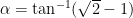
. , namely
  , and
, and  where this happens, I also note that
  ,
,  , and
, and  are increasing functions, and so
  lies in the interval
  . Likewise, to determine where
  .
.
 and
and  , I obtain
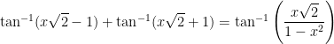
![\tan \left[ \tan^{-1} ( x\sqrt{2} - 1 ) + \tan^{-1}( x \sqrt{2} + 1) \right] = \displaystyle \frac{x \sqrt{2} - 1 + x \sqrt{2} + 1}{1 - (x\sqrt{2} - 1)(x\sqrt{2} + 1)}](https://s0.wp.com/latex.php?latex=%5Ctan+%5Cleft%5B+%5Ctan%5E%7B-1%7D+%28+x%5Csqrt%7B2%7D+-+1+%29+%2B+%5Ctan%5E%7B-1%7D%28+x+%5Csqrt%7B2%7D+%2B+1%29+%5Cright%5D+%3D+%5Cdisplaystyle+%5Cfrac%7Bx+%5Csqrt%7B2%7D+-+1+%2B+x+%5Csqrt%7B2%7D+%2B+1%7D%7B1+-+%28x%5Csqrt%7B2%7D+-+1%29%28x%5Csqrt%7B2%7D+%2B+1%29%7D&bg=ffffff&fg=000000&s=0&c=20201002)


 .
.
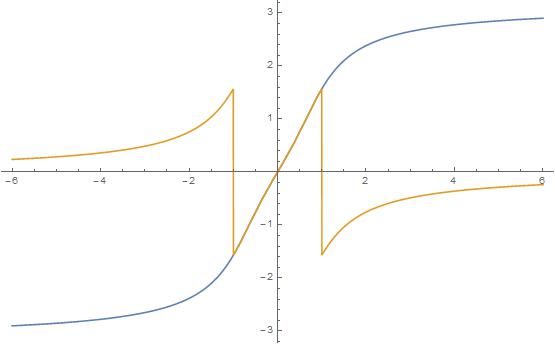
 that depends on
  and
and  have different graphs. (The vertical lines in the orange graph indicate where the right-hand side is undefined when
  :
:


 .
.

 and
and  , I can continue:
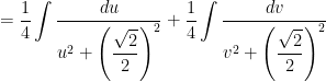


 :
: