In my capstone class for future secondary math teachers, I ask my students to come up with ideas for engaging their students with different topics in the secondary mathematics curriculum. In other words, the point of the assignment was not to devise a full-blown lesson plan on this topic. Instead, I asked my students to think about three different ways of getting their students interested in the topic in the first place.
I plan to share some of the best of these ideas on this blog (after asking my students’ permission, of course).
This student submission comes from my former student Andrew Sansom. His topic, from Algebra II: solving linear systems of equations with matrices.

A1. What interesting (i.e., uncontrived) word problems using this topic can your students do now? (You may find resources such as http://www.spacemath.nasa.gov to be very helpful in this regard; feel free to suggest others.)
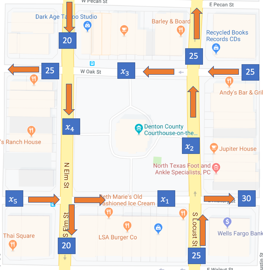
The Square in Downtown Denton is a popular place to visit and hang out. A new business owner needs to decide which road he should put an advertisement so that the most people will see it as they drive by. He does not have enough resources to traffic every block and street, but he knows that he can use algebra to solve for the ones he missed. In the above map, he put a blue box that contains the number of people that walked on each street during one hour. Use a system of linear equations to determine how much traffic is on every street/block on this map.
HINT: Remember that in every intersection, the same number of people have to walk in and walk out each hour, so write an equation for each intersection that has the sum of people walking in is equal to the number of people walking out.
HINT: Remember that the same people enter and exit the entire map every hour. Write an equation that has the sum of each street going into the map equal to the sum of each street going out of the map.
Solution:
1. Build each equation, as suggested by the hints.
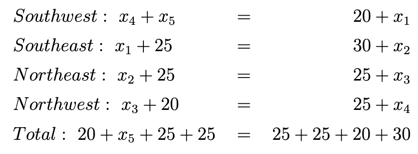
2. Rewrite the system of simultaneous linear equations in standard form.

3. Rewrite the system as an augmented matrix
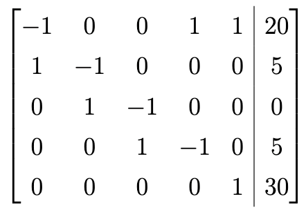
4. Reduce the system to Reduced Row Echelon Form (using a calculator)
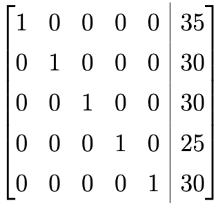
5. Use this reduced matrix to find solutions for each variable
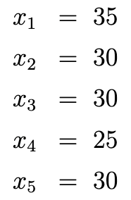
This gives us a completed map:

Clearly, the business owner should advertise on Hickory Street between Elm and Locust St (Possibly in front of Beth Marie’s).
B1. How can this topic be used in your students’ future courses in mathematics or science?
Systems of Simultaneous Linear Equations appear frequently in most problems that involve modelling more than one thing at a time. In high school, the ability to use matrices to solve such systems (especially large ones) simply many problems that would appear in AP or IB Physics exams. Circuit Analysis (including Kirchhof’s and Ohm’s laws) frequently amounts to setting up large systems of simultaneous equations similar to the above network traffic problem. Similarly, there are kinematics problems where multiple forces/torques acting on an object that naturally lend themselves to large systems of equations.
In chemistry, mixture problems can be solved using systems of equations. If more than substance is being mixed, then the system can become too large to efficiently solve except by Gaussian Elimination and matrix operations. (DeFreese, n.d.)
At the university level, learning to solve systems using matrices prepares the student for Linear Algebra, which is useful in almost every math class taken thereafter.
D4. What are the contributions of various cultures to this topic?
Simultaneous linear equations were featured in Ancient China in a text called Jiuzhang Suanshu or Nine Chapters of the Mathematical Art to solve problems involving weights and quantities of grains. The method prescribed involves listing the coefficients of terms in an array is exceptionally similar to Gaussian Elimination.
Later, in early modern Europe, the methods of elimination were known, but not taught in textbooks until Newton published such an English text in 1720, though he did not use matrices in that text. Gauss provided an even more systematic approach to solving simultaneous linear equations involving least squares by 1794, which was used in 1801 to find Ceres when it was sighted and then lost. During Gauss’s lifetime and in the century that followed, Gauss’s method of elimination because a standard way of solving large systems for human computers. Furthermore, by adopting brackets, “Gauss relieved computers of the tedium of having to rewrite equations, and in so doing, he enabled them to consider how to best organize their work.” (Grcar J. F., 2011).
The use of matrices in elimination appeared in 1895 with Wilhelm Jordan and 1888 by B.I. Clasen. Since then, the method we use today has become commonly attributed to Jordan and commemorated with the name “Gauss-Jordan Method”.
References:
DeFreese, C. (n.d.). Mixture Problems. Retrieved from University of Missouri-St. Louis–Department of Mathematics and Computer Science: http://www.umsl.edu/~defreeseca/intalg/ch8extra/mixture.htm
Grcar, J. F. (2011, May). Historia Mathematica–How ordinary elimination became Gaussian elimination. Retrieved from ScienceDirect: https://www.sciencedirect.com/science/article/pii/S0315086010000376
Grcar, J. F. (n.d.). Mathematics of Gaussian Elimination. Retrieved from American Mathematical Society: https://www.ams.org/notices/201106/rtx110600782p.pdf


 ,
, and
and  . With no modesty, I call this one the Quintanilla sequence when I teach my students — the forgotten little brother of the Fibonacci sequence.
 , we obtain the characteristic equation


 ,
, and
and  are constants to be determined. To find these constants, we plug in
  :
: .
. :
: .
.

 and
and  , so that
 ,
,
 ,
,


 , or
, or  .
. and
and  . The second and third equations then become
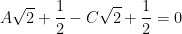
 ,
, ,
, , so that
  and
and  .
.

 is independent of
  , I’ll now give a fourth method.
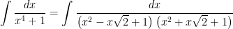
 yields the following simplification:


![= \displaystyle \int_{-\infty}^{\infty} \frac{ 2(1+u^2) du}{ ([u - \sqrt{1-b^2}]^2 +b^2)([u + \sqrt{1-b^2}]^2 +b^2}](https://s0.wp.com/latex.php?latex=%3D+%5Cdisplaystyle+%5Cint_%7B-%5Cinfty%7D%5E%7B%5Cinfty%7D+%5Cfrac%7B+2%281%2Bu%5E2%29+du%7D%7B+%28%5Bu+-+%5Csqrt%7B1-b%5E2%7D%5D%5E2+%2Bb%5E2%29%28%5Bu+%2B+%5Csqrt%7B1-b%5E2%7D%5D%5E2+%2Bb%5E2%7D&bg=ffffff&fg=000000&s=0&c=20201002)
![\displaystyle \int_{-\infty}^{\infty} \left[ \frac{1}{[u - \sqrt{1-b^2}]^2 +b^2} + \frac{1}{[u + \sqrt{1-b^2}]^2 +b^2} \right] du](https://s0.wp.com/latex.php?latex=%5Cdisplaystyle+%5Cint_%7B-%5Cinfty%7D%5E%7B%5Cinfty%7D+%5Cleft%5B+%5Cfrac%7B1%7D%7B%5Bu+-+%5Csqrt%7B1-b%5E2%7D%5D%5E2+%2Bb%5E2%7D+%2B+%5Cfrac%7B1%7D%7B%5Bu+%2B+%5Csqrt%7B1-b%5E2%7D%5D%5E2+%2Bb%5E2%7D+%5Cright%5D+du&bg=ffffff&fg=000000&s=0&c=20201002)
 . (The cases
  and
and  have already been handled earlier in this series.)
 .
.![Q = \displaystyle \left[ \frac{1}{|b|} \tan^{-1} \left( \frac{u - \sqrt{1-b^2}}{b} \right) + \frac{1}{|b|} \tan^{-1} \left( \frac{u - \sqrt{1-b^2}}{b} \right) \right]^{\infty}_{-\infty}](https://s0.wp.com/latex.php?latex=Q+%3D+%5Cdisplaystyle+%5Cleft%5B+%5Cfrac%7B1%7D%7B%7Cb%7C%7D+%5Ctan%5E%7B-1%7D+%5Cleft%28+%5Cfrac%7Bu+-+%5Csqrt%7B1-b%5E2%7D%7D%7Bb%7D+%5Cright%29+%2B+%5Cfrac%7B1%7D%7B%7Cb%7C%7D+%5Ctan%5E%7B-1%7D+%5Cleft%28+%5Cfrac%7Bu+-+%5Csqrt%7B1-b%5E2%7D%7D%7Bb%7D+%5Cright%29+%5Cright%5D%5E%7B%5Cinfty%7D_%7B-%5Cinfty%7D&bg=ffffff&fg=000000&s=0&c=20201002)
![= \displaystyle \frac{1}{|b|} \left[ \left( \frac{\pi}{2} + \frac{\pi}{2} \right) - \left( \frac{-\pi}{2} + \frac{-\pi}{2} \right) \right]](https://s0.wp.com/latex.php?latex=%3D+%5Cdisplaystyle+%5Cfrac%7B1%7D%7B%7Cb%7C%7D+%5Cleft%5B+%5Cleft%28+%5Cfrac%7B%5Cpi%7D%7B2%7D+%2B+%5Cfrac%7B%5Cpi%7D%7B2%7D+%5Cright%29+-+%5Cleft%28+%5Cfrac%7B-%5Cpi%7D%7B2%7D+%2B+%5Cfrac%7B-%5Cpi%7D%7B2%7D+%5Cright%29+%5Cright%5D&bg=ffffff&fg=000000&s=0&c=20201002)
 .
.![\displaystyle \frac{ 2(1+u^2)}{ ([u - \sqrt{1-b^2}]^2 +b^2)([u + \sqrt{1-b^2}]^2 +b^2)} = \displaystyle \frac{Au + B}{[u - \sqrt{1-b^2}]^2 +b^2} + \frac{Cu + D}{[u + \sqrt{1-b^2}]^2 +b^2}](https://s0.wp.com/latex.php?latex=%5Cdisplaystyle+%5Cfrac%7B+2%281%2Bu%5E2%29%7D%7B+%28%5Bu+-+%5Csqrt%7B1-b%5E2%7D%5D%5E2+%2Bb%5E2%29%28%5Bu+%2B+%5Csqrt%7B1-b%5E2%7D%5D%5E2+%2Bb%5E2%29%7D+%3D+%5Cdisplaystyle+%5Cfrac%7BAu+%2B+B%7D%7B%5Bu+-+%5Csqrt%7B1-b%5E2%7D%5D%5E2+%2Bb%5E2%7D+%2B+%5Cfrac%7BCu+%2B+D%7D%7B%5Bu+%2B+%5Csqrt%7B1-b%5E2%7D%5D%5E2+%2Bb%5E2%7D&bg=ffffff&fg=000000&s=0&c=20201002) ,
,![\displaystyle \frac{ 2(1+u^2)}{ ([u - \sqrt{1-b^2}]^2 +b^2)([u + \sqrt{1-b^2}]^2 +b^2)} = \displaystyle \frac{Au + B}{u^2 - 2u \sqrt{1-b^2} +1} + \frac{Cu + D}{u^2 + 2u\sqrt{1-b^2} + 1}](https://s0.wp.com/latex.php?latex=%5Cdisplaystyle+%5Cfrac%7B+2%281%2Bu%5E2%29%7D%7B+%28%5Bu+-+%5Csqrt%7B1-b%5E2%7D%5D%5E2+%2Bb%5E2%29%28%5Bu+%2B+%5Csqrt%7B1-b%5E2%7D%5D%5E2+%2Bb%5E2%29%7D+%3D+%5Cdisplaystyle+%5Cfrac%7BAu+%2B+B%7D%7Bu%5E2+-+2u+%5Csqrt%7B1-b%5E2%7D+%2B1%7D+%2B+%5Cfrac%7BCu+%2B+D%7D%7Bu%5E2+%2B+2u%5Csqrt%7B1-b%5E2%7D+%2B+1%7D&bg=ffffff&fg=000000&s=0&c=20201002) .
.


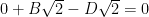
 and matching coefficients yields the following system of four equations in four unknowns:


 .
.


 ,
, as well. Finally, from the second equation, I see that

 ,
, as well. This yields the partial fractions decomposition
![\displaystyle \frac{ 2(1+u^2)}{ ([u - \sqrt{1-b^2}]^2 +b^2)([u + \sqrt{1-b^2}]^2 +b^2)} = \displaystyle \frac{1}{[u - \sqrt{1-b^2}]^2 +b^2} + \frac{1}{[u + \sqrt{1-b^2}]^2 +b^2}](https://s0.wp.com/latex.php?latex=%5Cdisplaystyle+%5Cfrac%7B+2%281%2Bu%5E2%29%7D%7B+%28%5Bu+-+%5Csqrt%7B1-b%5E2%7D%5D%5E2+%2Bb%5E2%29%28%5Bu+%2B+%5Csqrt%7B1-b%5E2%7D%5D%5E2+%2Bb%5E2%29%7D+%3D+%5Cdisplaystyle+%5Cfrac%7B1%7D%7B%5Bu+-+%5Csqrt%7B1-b%5E2%7D%5D%5E2+%2Bb%5E2%7D+%2B+%5Cfrac%7B1%7D%7B%5Bu+%2B+%5Csqrt%7B1-b%5E2%7D%5D%5E2+%2Bb%5E2%7D&bg=ffffff&fg=000000&s=0&c=20201002) .
.![\displaystyle \frac{1}{[u - \sqrt{1-b^2}]^2 +b^2} + \frac{1}{[u + \sqrt{1-b^2}]^2 +b^2}](https://s0.wp.com/latex.php?latex=%5Cdisplaystyle+%5Cfrac%7B1%7D%7B%5Bu+-+%5Csqrt%7B1-b%5E2%7D%5D%5E2+%2Bb%5E2%7D+%2B+%5Cfrac%7B1%7D%7B%5Bu+%2B+%5Csqrt%7B1-b%5E2%7D%5D%5E2+%2Bb%5E2%7D&bg=ffffff&fg=000000&s=0&c=20201002)
![= \displaystyle \frac{[u + \sqrt{1-b^2}]^2 +b^2 + [u - \sqrt{1-b^2}]^2 +b^2}{([u - \sqrt{1-b^2}]^2 +b^2)([u + \sqrt{1-b^2}]^2 +b^2)}](https://s0.wp.com/latex.php?latex=%3D+%5Cdisplaystyle+%5Cfrac%7B%5Bu+%2B+%5Csqrt%7B1-b%5E2%7D%5D%5E2+%2Bb%5E2+%2B+%5Bu+-+%5Csqrt%7B1-b%5E2%7D%5D%5E2+%2Bb%5E2%7D%7B%28%5Bu+-+%5Csqrt%7B1-b%5E2%7D%5D%5E2+%2Bb%5E2%29%28%5Bu+%2B+%5Csqrt%7B1-b%5E2%7D%5D%5E2+%2Bb%5E2%29%7D&bg=ffffff&fg=000000&s=0&c=20201002)
![= \displaystyle \frac{u^2 + 2u\sqrt{1-b^2} + 1 - b^2 + b^2 + u^2 - 2u\sqrt{1-b^2} + 1 - b^2 + b^2}{([u - \sqrt{1-b^2}]^2 +b^2)([u + \sqrt{1-b^2}]^2 +b^2)}](https://s0.wp.com/latex.php?latex=%3D+%5Cdisplaystyle+%5Cfrac%7Bu%5E2+%2B+2u%5Csqrt%7B1-b%5E2%7D+%2B+1+-+b%5E2+%2B+b%5E2+%2B+u%5E2+-+2u%5Csqrt%7B1-b%5E2%7D+%2B+1+-+b%5E2+%2B+b%5E2%7D%7B%28%5Bu+-+%5Csqrt%7B1-b%5E2%7D%5D%5E2+%2Bb%5E2%29%28%5Bu+%2B+%5Csqrt%7B1-b%5E2%7D%5D%5E2+%2Bb%5E2%29%7D&bg=ffffff&fg=000000&s=0&c=20201002)
![= \displaystyle \frac{2u^2 + 2}{([u - \sqrt{1-b^2}]^2 +b^2)([u + \sqrt{1-b^2}]^2 +b^2)}](https://s0.wp.com/latex.php?latex=%3D+%5Cdisplaystyle+%5Cfrac%7B2u%5E2+%2B+2%7D%7B%28%5Bu+-+%5Csqrt%7B1-b%5E2%7D%5D%5E2+%2Bb%5E2%29%28%5Bu+%2B+%5Csqrt%7B1-b%5E2%7D%5D%5E2+%2Bb%5E2%29%7D&bg=ffffff&fg=000000&s=0&c=20201002) .
.![= \displaystyle \int_{-\infty}^{\infty} \left[ \displaystyle \left( \frac{2 - 2k_1^2}{k_2^2 - k_1^2} \right) \frac{1}{u^2 + k_1^2} + \displaystyle \left( \frac{2 k_2^2 - 2}{k_2^2 - k_1^2} \right) \frac{1}{u^2 + k_2^2} \right] du](https://s0.wp.com/latex.php?latex=%3D+%5Cdisplaystyle+%5Cint_%7B-%5Cinfty%7D%5E%7B%5Cinfty%7D+%5Cleft%5B+%5Cdisplaystyle+%5Cleft%28+%5Cfrac%7B2+-+2k_1%5E2%7D%7Bk_2%5E2+-+k_1%5E2%7D+%5Cright%29+%5Cfrac%7B1%7D%7Bu%5E2+%2B+k_1%5E2%7D+%2B+%5Cdisplaystyle+%5Cleft%28+%5Cfrac%7B2+k_2%5E2+-+2%7D%7Bk_2%5E2+-+k_1%5E2%7D+%5Cright%29+%5Cfrac%7B1%7D%7Bu%5E2+%2B+k_2%5E2%7D+%5Cright%5D+du&bg=ffffff&fg=000000&s=0&c=20201002) ,
, and
and  are the positive numbers so that
 ,
, ,
,
 ,
,![Q = \left[ \displaystyle \left( \frac{2 - 2k_1^2}{k_2^2 - k_1^2} \right) \frac{1}{k_1}\tan^{-1} \left( \frac{u}{k_1} \right) + \displaystyle \left( \frac{2 k_2^2 - 2}{k_2^2 - k_1^2} \right) \displaystyle \frac{1}{k_2} \tan^{-1} \left( \frac{u}{k_2} \right) \right]^{\infty}_{-\infty}](https://s0.wp.com/latex.php?latex=Q+%3D+%5Cleft%5B+%5Cdisplaystyle+%5Cleft%28+%5Cfrac%7B2+-+2k_1%5E2%7D%7Bk_2%5E2+-+k_1%5E2%7D+%5Cright%29+%5Cfrac%7B1%7D%7Bk_1%7D%5Ctan%5E%7B-1%7D+%5Cleft%28+%5Cfrac%7Bu%7D%7Bk_1%7D+%5Cright%29+%2B+%5Cdisplaystyle+%5Cleft%28+%5Cfrac%7B2+k_2%5E2+-+2%7D%7Bk_2%5E2+-+k_1%5E2%7D+%5Cright%29+%5Cdisplaystyle+%5Cfrac%7B1%7D%7Bk_2%7D+%5Ctan%5E%7B-1%7D+%5Cleft%28+%5Cfrac%7Bu%7D%7Bk_2%7D+%5Cright%29+%5Cright%5D%5E%7B%5Cinfty%7D_%7B-%5Cinfty%7D&bg=ffffff&fg=000000&s=0&c=20201002)


 .
.
 ,
,
 from the last equation. Therefore,


 ,
, for the cases
 is a real number for the four roots of the denominator.
 if
if  ,
,![\left[ 2|b| \sqrt{b^2-1} \right]^2 = 4b^2 (b^2 - 1) = 4b^4 - 4b^2](https://s0.wp.com/latex.php?latex=%5Cleft%5B+2%7Cb%7C+%5Csqrt%7Bb%5E2-1%7D+%5Cright%5D%5E2+%3D+4b%5E2+%28b%5E2+-+1%29+%3D+4b%5E4+-+4b%5E2&bg=ffffff&fg=000000&s=0&c=20201002) .
.![(2b^2 - 1)^2 > \left[ 2|b| \sqrt{b^2-1} \right]^2](https://s0.wp.com/latex.php?latex=%282b%5E2+-+1%29%5E2+%3E+%5Cleft%5B+2%7Cb%7C+%5Csqrt%7Bb%5E2-1%7D+%5Cright%5D%5E2&bg=ffffff&fg=000000&s=0&c=20201002)


 ,
, ,
, and not
  . However, there are no
  and
and  terms in the denominator, I can treat
  , I clear out the denominator:
![2u^2 + 2 = A \left[ u^2 + k_2^2 \right] + B \left[ u^2 + k_1^2 \right]](https://s0.wp.com/latex.php?latex=2u%5E2+%2B+2+%3D+A+%5Cleft%5B+u%5E2+%2B+k_2%5E2+%5Cright%5D+%2B+B+%5Cleft%5B+u%5E2+%2B+k_1%5E2+%5Cright%5D&bg=ffffff&fg=000000&s=0&c=20201002)


 into the second equation, I get


 Part 1