Confirming Einstein’s Theory of General Relativity With Calculus, Part 3: Method of Successive Approximations

In this series, I’m discussing how ideas from calculus and precalculus (with a touch of differential equations) can predict the precession in Mercury’s orbit and thus confirm Einstein’s theory of general relativity. The origins of this series came from a class project that I assigned to my Differential Equations students maybe 20 years ago.

One technique that will be necessary for this confirmation is the method of successive approximations. This will be needed in the context of a differential equation; however, we can illustrate the concept by finding the roots of a polynomial. Consider the quadratic equation

$x^2 - x - 1 = 0$ .

(Naturally, we can solve for $x$ using the quadratic formula; more on that later.) To apply the method of successive approximation, we will rewrite this so that $x$ appears on the left side and some function of $x$ appears on the right side. I will choose

$x^2 = x + 1$ , or

$x = 1 + \displaystyle \frac{1}{x}$ .

Here’s the idea of the method of successive approximations to obtain a recursively defined sequence that (hopefully) convergence to a solution of this equation:

Start with an initial guess $x_0$ .
Plug $x_0$ into the right-hand side to get a new guess, $x_1$ .
Plug $x_1$ into the right-hand side to get a new guess, $x_2$ .
And repeat.

For example, suppose that we choose $x_0 = 1$ . Then

$x_1 = 1 + \displaystyle \frac{1}{x_0} = 1 + \displaystyle \frac{1}{1} = 2$

$x_2 = 1 + \displaystyle \frac{1}{x_1} = 1 + \displaystyle \frac{1}{2} = \displaystyle \frac{3}{2} = 1.5$

$x_3 = 1 + \displaystyle \frac{1}{x_2} = 1 + \displaystyle \frac{1}{3/2} = \displaystyle \frac{5}{3} \approx 1.667$

$x_4 = 1 + \displaystyle \frac{1}{x_3} = 1 + \displaystyle \frac{1}{5/3} = \displaystyle \frac{8}{5} = 1.6$

$x_5 = 1 + \displaystyle \frac{1}{x_4} = 1 + \displaystyle \frac{1}{8/5} = \displaystyle \frac{13}{8} = 1.625$

$x_6 = 1 + \displaystyle \frac{1}{x_5} = 1 + \displaystyle \frac{1}{13/8} = \displaystyle \frac{21}{13} \approx 1.615$

$x_7 = 1 + \displaystyle \frac{1}{x_6} = 1 + \displaystyle \frac{1}{21/13} = \displaystyle \frac{34}{21} \approx 1.619$

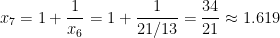
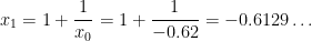
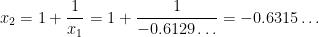
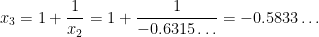
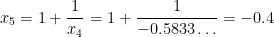
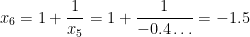
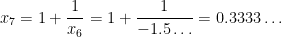
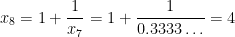
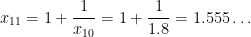
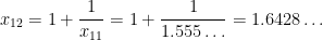
This sequence can be computed by entering $1$ into a calculator, then entering $1 + 1 \div \hbox{Ans}$ , and then repeatedly hitting the $=$ button.

We see that the sequence appears to be converging to something, and that something is a root of the equation $x^2 - x - 1 = 0$ , which we now find via the quadratic formula:

$x = \displaystyle \frac{1 \pm \sqrt{1 - 4 \cdot 1 \cdot (-1)}}{2} = \frac{1 \pm \sqrt{5}}{2}$ .

So it looks like the above sequence is converging to the positive root $(1 + \sqrt{5})/2 \approx 1.618$ .

(Parenthetically, you might notice that the Fibonacci sequence appears in the numerators and denominators of this sequence. As you might guess, that’s not a coincidence.)

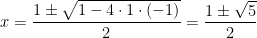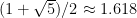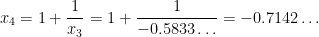
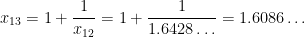
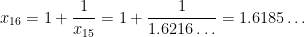
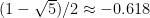Like most numerical techniques, this method doesn’t always work like we think it would. Another solution is the negative root $(1 - \sqrt{5})/2 \approx -0.618$ . Unfortunately, if we start with a guess near this root, like $x_0 = -0.62$ , the sequence unexpectedly diverges from $-0.618\dots$ but eventually converges to the positive root $1.618\dots$ :

$x_1 = 1 + \displaystyle \frac{1}{x_0} = 1 + \displaystyle \frac{1}{-0.62} = -0.6129\dots$

$x_2 = 1 + \displaystyle \frac{1}{x_1} = 1 + \displaystyle \frac{1}{-0.6129\dots} = -0.6315\dots$

$x_3 = 1 + \displaystyle \frac{1}{x_2} = 1 + \displaystyle \frac{1}{-0.6315\dots} = -0.5833\dots$

$x_4 = 1 + \displaystyle \frac{1}{x_3} = 1 + \displaystyle \frac{1}{-0.5833\dots} = -0.7142\dots$

$x_5 = 1 + \displaystyle \frac{1}{x_4} = 1 + \displaystyle \frac{1}{-0.5833\dots} = -0.4$

$x_6 = 1 + \displaystyle \frac{1}{x_5} = 1 + \displaystyle \frac{1}{-0.4\dots} = -1.5$

$x_7 = 1 + \displaystyle \frac{1}{x_6} = 1 + \displaystyle \frac{1}{-1.5\dots} = 0.3333\dots$

$x_8 = 1 + \displaystyle \frac{1}{x_7} = 1 + \displaystyle \frac{1}{0.3333\dots} = 4$

$x_9 = 1 + \displaystyle \frac{1}{x_8} = 1 + \displaystyle \frac{1}{4} = 1.25$

$x_{10} = 1 + \displaystyle \frac{1}{x_9} = 1 + \displaystyle \frac{1}{1.25} = 1.8$

$x_{11} = 1 + \displaystyle \frac{1}{x_{10}} = 1 + \displaystyle \frac{1}{1.8} = 1.555\dots$

$x_{12} = 1 + \displaystyle \frac{1}{x_{11}} = 1 + \displaystyle \frac{1}{1.555\dots} = 1.6428\dots$

$x_{13} = 1 + \displaystyle \frac{1}{x_{12}} = 1 + \displaystyle \frac{1}{1.6428\dots} = 1.6086\dots$

$x_{14} = 1 + \displaystyle \frac{1}{x_{13}} = 1 + \displaystyle \frac{1}{1.6086\dots} = 1.6216\dots$

$x_{15} = 1 + \displaystyle \frac{1}{x_{14}} = 1 + \displaystyle \frac{1}{1.6216\dots} = 1.6166\dots$

$x_{16} = 1 + \displaystyle \frac{1}{x_{15}} = 1 + \displaystyle \frac{1}{1.6216\dots} = 1.6185\dots$

I should note that the method of successive approximations generally converges at a slower pace than Newton’s method. However, this method will be good enough when we use it to predict the precession in Mercury’s orbit.

Engaging students: Arithmetic series

In my capstone class for future secondary math teachers, I ask my students to come up with ideas for engaging their students with different topics in the secondary mathematics curriculum. In other words, the point of the assignment was not to devise a full-blown lesson plan on this topic. Instead, I asked my students to think about three different ways of getting their students interested in the topic in the first place.

I plan to share some of the best of these ideas on this blog (after asking my students’ permission, of course).

This student submission comes from my former student Eduardo Torres Manzanarez. His topic, from Precalculus: arithmetic series.

A1) What interesting (i.e., uncontrived) word problems using this topic can your students do now?

One interesting word problem to ask students to get them thinking about the idea of an arithmetic series, specifically a finite arithmetic series, is to have students come up with the total sum of the first 100 positive integers larger than 0 (i.e., 1 to 100) without actually adding all the integers up. Students will probably not figure out the total sum without adding the integers up one by one but if students are shown these numbers physically as cards labeled then a few might notice that the numbers taken at each end form pairs that add to the same sum. Turns out that the total sum is the number of pairs multiplied by 101. It can be explained to students that the 101 results from taking the first term and the last term (i.e., 1 and 100) and seeing that the sum is 101. This is true when we add 2 and 99, 3 and 98, 4, and 97, and so on. Hence, we will have 50 pairs since we have 100 numbers and so we have 50*101 as our sum. This problem can be extended to the story Gauss and how he apparently solved this problem as a child relatively fast and the teacher pointed out this question to them because he was apparently lazy. Now, this can be extended to adding all the integers from 1 to 200 and so on and having students come up with a general formula. Students can then think about an odd number of integers and see if that formula holds. Lastly, the connection between adding a number of terms with the same difference between each term is defined as an arithmetic series and so all the problems they have been doing are arithmetic problems in disguise.

B2) How can this topic be used in your students’ future courses in mathematics and science?

This topic is heavily used when discussing convergence in calculus. It provides insight into the validity that every series has a total sum that can be written as a number. Turns out this is true for all series that are finite but when discussing infinite series, it can be true of false that it converges to an actual value. So, students will have to ponder this idea for infinite arithmetic series in the future. Also, arithmetic series can be used to model certain situations in science within biology and physics. Thinking about arithmetic series provides information in tackling other types of series such as geometric in terms of behavior and solution. How does a geometric series behave? Well, each term increases with a common ratio instead of a common addition. Does the finite series converge? Yes, we know that every finite series does and this one basically behaves like the arithmetic in which we can easily find the total sum using a formula. Does the infinite series converge? Well, just like an arithmetic series it depends on the situation and the terms within the problem.

C1) How has this topic appeared in pop culture (movies, TV, current music, video games, etc.)?

This topic has appeared in a particular movie called “All Quiet on the Western Front” which was released in 1930 and is an adaption of the novel that was published in 1929 by Erich Remarque. Within this movie, there is a scene in which a soldier states the formula for finding the sum of an arithmetic series. The soldier specifically states the formula S = A + N*(L / 2) and this corresponds to arithmetic series in accordance with the area of a rectangle and the area of a triangle. This is in a way a longer version of the short-hand formula we use today. One particular statement made from the soldier is that he mentions how beautiful the formula is. For some students, they can probably relate to the idea that something so complicated as adding 100000 terms that have a constant difference can be found using a short formula. Many problems in mathematics seem complicated at first in accordance with doing “grunt work” but many of them have beautiful solutions to them.

Engaging students: Arithmetic sequences

I plan to share some of the best of these ideas on this blog (after asking my students’ permission, of course).

This student submission comes from my former student Danielle Pope. Her topic, from Precalculus: arithmetic sequences.

How can this topic be used in your students’ future courses in mathematics or science?

In the future, the topic of arithmetic sequences will be built upon by introducing another sequence, the geometric sequence. A geometric sequence is just a sequence of multiples instead of increasing by a constant. The next topic introduced will be finding the sum of a sequence of numbers. This will be introduced as a series. The summation symbol will also be introduced to kids and they will learn that new notation. Summations will bring along many formulas for finding the leading coefficient and will show up later in Calculus 2 classes when talking about convergence and divergence of series. Another one of the things that kids will always be doing with sequences and series is finding the general form of a given sequence or series. Through school, this idea will never change the sequence and series will just get harder to identify.

What interesting things can you say about the people who contributed to the discovery and/or the development of this topic? (You might want to consult Math Through The Ages.)

An arithmetic sequence is a set of numbers that have a constant difference between each term. One of the main people that come up when researching these sequences is Carl Friedrich Gauss. Many math-loving people know him as the “Prince of mathematicians”. He is famous for coming up with the equations to solve the sum of an arithmetic sequence. This comes as no surprise that he came up with this formula. The surprising thing about this realization is that he made it at an age young enough to still be in grade school. Stories say that Gauss was asked to solve for the sum on the board in grade school and used the formula of M ( M + 1 ) / 2 to solve for the correct answer. This just goes to show that anyone can, in fact, contribute to the greater good of mathematics at any age.

How have different cultures throughout time used this topic in their society?

One of the first civilizations that utilized sequences was the Egyptians. They used the sequence of multiples of 2 to do their multiplication. The basic sequence is 1, 2, 4, 8, 16, 32, … and we are trying to solve 24 x 13 with the process pictured below.

The process behind this is to write the multiple of 2 sequences down the left side of the paper until you reach the largest multiple of 2 without going over the second number being multiplied, in this case, 13. Once that is done set the first term on the right side equal to the first number being multiplied, in this case, 24. Next, multiply the right side by 4 until you get the same amount of terms on the left side. Lastly find the sum of numbers on the left that add to 13, which are 1, 4, and 8. Add the corresponding multiples from the side, 24 + 96 + 192 = 312. The right side sum of the corresponding numbers checked on the left gives the product of the original problem, i.e. 312. This trick is cool to show just on its own but it’s also cool because it uses something as simple as a specific list of numbers aka a sequence of numbers.

References

http://www.softschools.com/facts/scientists/carl_friedrich_gauss_facts/827/

https://rabungapalgebraiii.wikispaces.com/Arithmetic+Sequences+and+Series

Click to access egyptian_arithmetic.pdf

Engaging students: Arithmetic sequences

I plan to share some of the best of these ideas on this blog (after asking my students’ permission, of course).

This student submission comes from my former student Jessica Martinez. Her topic, from Precalculus: arithmetic sequences.

What interesting things can you say about the people who contributed to the discovery and/or the development of this topic?

Perhaps some of us realized that we were pretty good at math at a young age, though I wonder if anyone was as good at math, or as fast a learner, as Carl Friedrich Gauss was. When Gauss was two he taught himself how to read; when he was three he checked and corrected his dad’s math whenever his father was calculating the payroll; and probably one of the most famous stories about Gauss was that when he was 9 or 10 he created a formula for an arithmetic progression just by glancing at a problem, which ultimately helped Gauss to start his lifelong education and career in mathematical theory. Gauss was sitting in an arithmetic class taught by a man named Buttner, who was said to dislike teaching peasant children, but he was so surprised and impressed that Gauss correctly calculated the solution to the sequence problem that Buttner started to take Gauss under his and wing and help him with his education. Turns out that the formula created by Gauss can be used to find any arithmetic progression. Later on, Gauss eventually earned a doctorate at the age of 22 with the financial help of the Duke of Brunswick; his dissertation was about the fundamental theory of algebra. Gauss had numerous and important contributions to the field of mathematics, but I won’t state them here for the fear of feeling highly insignificant to one of the greatest mathematicians of all time.

How has this topic appeared in pop culture (movies, TV, current music, video games, etc.)?

This is kind of a cool tidbit for any music lovers and any Led Zeppelin fans. So Led Zeppelin III had a crazy array of imagery on its album sleeve and volvelle, which was great way to further engage people who listened to their music. However, we know that records are a thing of past, replaced by CDs and now online streaming. So a musician named Bill Baird, who was inspired by the themes of Led Zeppelin’s third album, created a way to make his website and album just as aesthetically pleasing and interesting as LZ by using mathematical equations and formulas. The site where you can listen to his music has a sort of kaleidoscope design (inspired by LZ’s sundials and astronomical designs) that changes as the music plays, where the artwork “mimics the music” since music themes and sounds are constantly changing over time. However, even more interesting is that the music is different for every listener. The site uses an arithmetic sequence formula based on the listener’s location and the time they accessed the site along with the hand-mixed tracks by Bill to create a unique sequence (and thus a unique album) for every listener. If the database creates an already used track, it starts the process over again until it gets a new sequence.

How could you as a teacher create an activity or project that involves your topic?

One of my previous teachers suggested this as a great real world problem for arithmetic sequences: Halley’s Comet. The video itself is just a short clip in order to grab my students’ attention; the video describes the comet’s path, its velocity, and its appearances in history with fancy graphics and imaging which can appeal to the science and space lovers in my class along with history lovers. The path of the comet brings it around visible to earth about every 75 years. After we covered some basics on arithmetic sequences, I can present this video to my class and have them research the comet and how it can be represented with a sequence. Some of the questions I could ask them to answer could be: when did it last come? What are the next 3, 4, 5, etc. years it will visit? Have you or will you see it in your lifetime? Calculate its 50^th visit from its last visit, its 100^th visit? I could then challenge them to find some other natural phenomena that also follows an arithmetic sequence.

References

[Video file]. (2015, January 10). In The Legacy of Halley’s Comet. Retrieved November 18, 2016, from https://youtu.be/elsRH_utRdo

Carl Friedrich Gauss. (n.d.). Retrieved November 18, 2016, from http://www.sonoma.edu/math/faculty/falbo/gauss.html

Dial, C. (2016, October 27). Album Turns Into Something New Each Time It’s Played. Retrieved November 18, 2016, from http://www.psfk.com/2016/10/music-album-bill-baird-algorithm.html

Gauss: The Prince of Mathematics | Brilliant Math & Science Wiki. (n.d.). Retrieved November 18, 2016, from https://brilliant.org/wiki/gauss-the-prince-of-mathematics/

Howell, E. (2013, February 20). Halley’s Comet: Facts About the Most Famous Comet. Retrieved November 18, 2016, from http://www.space.com/19878-halleys-comet.html

My Favorite One-Liners: Part 28

In this series, I’m compiling some of the quips and one-liners that I’ll use with my students to hopefully make my lessons more memorable for them. Today’s quip is one that I’ll use when simple techniques get used in a complicated way.

Consider the solution of the linear recurrence relation

$Q_n = Q_{n-1} + 2 Q_{n-2}$ ,

where $F_0 = 1$ and $F_1 = 1$ . With no modesty, I call this one the Quintanilla sequence when I teach my students — the forgotten little brother of the Fibonacci sequence.

To find the solution of this linear recurrence relation, the standard technique — which is a pretty long procedure — is to first solve the characteristic equation, from $Q_n - Q_{n-1} - 2 Q_{n-2} = 0$ , we obtain the characteristic equation

$r^2 - r - 2 = 0$

This can be solved by any standard technique at a student’s disposal. If necessary, the quadratic equation can be used. However, for this one, the left-hand side simply factors:

$(r-2)(r+1) = 0$

$r=2 \qquad \hbox{or} \qquad r = -1$

(Indeed, I “developed” the Quintanilla equation on purpose, for pedagogical reasons, because its characteristic equation has two fairly simple roots — unlike the characteristic equation for the Fibonacci sequence.)

From these two roots, we can write down the general solution for the linear recurrence relation:

$Q_n = \alpha_1 \times 2^n + \alpha_2 \times (-1)^n$ ,

where $\alpha_1$ and $\alpha_2$ are constants to be determined. To find these constants, we plug in $n =0$ :

$Q_0 = \alpha_1 \times 2^0 + \alpha_2 \times (-1)^0$ .

To find these constants, we plug in $n =0$ :

$Q_0 = \alpha_1 \times 2^0 + \alpha_2 \times (-1)^0$ .

We then plug in $n =1$ :

$Q_1 = \alpha_1 \times 2^1 + \alpha_2 \times (-1)^1$ .

Using the initial conditions gives

$1 = \alpha_1 + \alpha_2$

$1 = 2 \alpha_1 - \alpha_2$

This is a system of two equations in two unknowns, which can then be solved using any standard technique at the student’s disposal. Students should quickly find that $\alpha_1 = 2/3$ and $\alpha_2 = 1/3$ , so that

$Q_n = \displaystyle \frac{2}{3} \times 2^n + \frac{1}{3} \times (-1)^n = \frac{2^{n+1} + (-1)^n}{3}$ ,

which is the final answer.

Although this is a long procedure, the key steps are actually first taught in Algebra I: solving a quadratic equation and solving a system of two linear equations in two unknowns. So here’s my one-liner to describe this procedure:

This is just an algebra problem on steroids.

Yes, it’s only high school algebra, but used in a creative way that isn’t ordinarily taught when students first learn algebra.

I’ll use this “on steroids” line in any class when a simple technique is used in an unusual — and usually laborious — way to solve a new problem at the post-secondary level.

Fibonacci convention

Source: https://www.facebook.com/Mathhappiness/photos/a.170688796611683.1073741829.101136273566936/321994341481127/?type=3&theater

Lychrel Numbers

A friend of mine posted the following on Facebook (with names redacted):

So [my daughter] comes home with this assignment:

For each number from 10 – 99, carry out the following process.

If the number is a palindrome (e.g., 77), stop.

Else reverse the number and add that to the original. E.g.: 45+54 = 99.

If the result is not a palindrome, repeat step (2) with the result.

Record the final palindromic result and the number of steps taken.

Most are simple.

56 + 65 = 110

110 + 011 = 121

Stop. 2 steps taken.

The numbers 89 and 98 were given for extra credit, and they mysteriously explode, taking 24 steps. It made [my daughter] cry.

She wanted me to check her work, so I decided it was a good time to teach the wonders of Python, and we very quickly had a couple of simple functions to do the trick.

Well, you saw where this was going. How many steps does 887 take?

We’re up to 104000 steps so far, and Python is crying.

True or false: For a given n, the above algorithm completes in finite time?

I guess I’ve been living under a rock for the past 20 years, because I had never heard of this problem before. It turns out that numbers not known to lead to a palindrome are called Lychrel numbers. However, no number in base-10 has been proven to be a Lychrel number. The first few candidate Lychrel numbers (i.e., numbers that have not been proven to not be Lychrel numbers) are 196, 295, 394, 493, 592, 689, 691, 788, 790, 879, 887, 978, 986, 1495, 1497, 1585, 1587, 1675, 1677, 1765, 1767, 1855, 1857, 1945, 1947, 1997, 2494, 2496, 2584, 2586, 2674, 2676, 2764, 2766, 2854, 2856, 2944, 2946, 2996, 3493, 3495, 3583, 3585, 3673, 3675…

The above algorithm is called the 196-algorithm, after the smallest suspected Lychrel number.

For further reading, I suggest the following links and the references therein:

http://mathworld.wolfram.com/196-Algorithm.html

http://mathworld.wolfram.com/LychrelNumber.html

http://www.p196.org/

http://www.mathpages.com/home/kmath004/kmath004.htm (which contains a proof that 10110 is a Lychrel number in binary and that Lychrel numbers always exist in base $2^k$ )

http://en.wikipedia.org/wiki/Lychrel_number

Exponential growth and decay (Part 9): Amortization tables

This post is inspired by one of the questions that I pose to our future high school math teachers during our Friday question-and-answer sessions. In these sessions, I play the role of a middle- or high-school student who’s asking a tricky question to his math teacher. Here’s the question:

A student asks, “My father bought a house for $200,000 at 12% interest. He told me that by the time he finishes paying for the house, it will have cost him more than $500,000. How is that possible? 12% of $200,000 is only $24,000.”

Without fail, these future teachers don’t have a good response to this question. Indeed, my experience is that most young adults (including college students) have never used an amortization table, which is the subject of today’s post.

In the past few posts, we have considered the solution of the following recurrence relation, which is often used to model the payment of a mortgage or of credit-card debt:

$A_{n+1} = r A_n - k$

With this difference equation, the rate at which the principal is reduced can be simply computed using Microsoft Excel. This tool is called an amortization schedule or an amortization table; see E-How for the instructions of how to build one. Here’s a sample Excel spreadsheet that I’ll be illustrating below: Amortization schedule. My personal experience is that many math majors have never seen such a spreadsheet, even though they are familiar with compound interest problems and certainly have the mathematical tools to understand this spreadsheet.

Here’s a screen capture from the spreadsheet:

The terms of the loan are typed into Cells B1 (length of loan, in years), B2 (annual percentage rate), and B3 (initial principal). Cell B4 is computed from this information using the Microsoft Excel command $\hbox{PMT}$ :

$=\hbox{PMT}(\hbox{B2}/12,\hbox{B1}*12,-\hbox{B3})$

This is the amount that must be paid every month in order to pay off the loan in the prescribed number of years. Of course, there is a formula for this:

$M = \displaystyle \frac{Pr}{12 \displaystyle \left[1 - \left( 1 + \frac{r}{12} \right)^{-12t} \right]}$

I won’t go into the derivation of this formula here, as it’s a bit complicated. Notice that this formula does not include escrow, points, closing costs, etc. This is strictly the amount of money that’s needed to pay down the principal.

The table, beginning in Row 8 of the above picture, shows how quickly the principal will be paid off. In row 8, the interest that’s paid for that month is computed by

$=\hbox{B8} * \$ \hbox{B}\$\hbox{2}/12$

Therefore, the amount of the monthly payment that actually goes toward paying down the principal will be

$= \$\hbox{B}\$\hbox{4} - \hbox{C8}$

Column E provides an opportunity to pay something extra each month; more on this later. So, after taking into account the payments in columns D and E, the amount remaining on the loan is recorded in Cell F8:

$= \hbox{B8} - \hbox{D8} - \hbox{E8}$

This amount is then copied into Cell B9, and then the pattern can be filled down.

The yellow graph shows how quickly the balance of the loan is paid off over the length of the loan. A picture is worth a thousand words: in the initial years of the loan, most of the payments are gobbled up by the interest, and so the principal is paid off slowly. Only in the latter years of the loan is the principal paid off quickly.

So, it stands to reason that any extra payments in the initial months and years of the loan can do wonders for paying off the loan quickly. For example, here’s a screenshot of what happens if an extra $200/month is paid only in the first 12 months of the loan:

A definite bend in the graph is evident in the initial 12 months until the normal payment is resumed in month 13. As a result of those extra payments, the curve now intersects the horizontal axis around 340. In other words, 20 fewer months are required to pay off the loan. Stated another way, the extra payments in the first year cost an extra $\$200 \times 12 = \$2400$ . However, in the long run, those payments saved about $\$536.82 \times 20 \approx \$10,700$ !

Exponential growth and decay (Part 8): Paying off credit-card debt via recurrence relations

The following problem in differential equations has a very practical application for anyone who has either (1) taken out a loan to buy a house or a car or (2) is trying to pay off credit card debt. To my surprise, most math majors haven’t thought through the obvious applications of exponential functions as a means of engaging their future students, even though it is directly pertinent to their lives (both the students’ and the teachers’).

You have a balance of $2,000 on your credit card. Interest is compounded continuously with a rate of growth of 25% per year. If you pay the minimum amount of $50 per month (or $600 per year), how long will it take for the balance to be paid?

In previous posts, I approached this problem using differential equations. There’s another way to approach this problem that avoids using calculus that, hypothetically, is within the grasp of talented Precalculus students. Instead of treating this problem as a differential equation, we instead treat it as a first-order difference equation (also called a recurrence relation):

$A_{n+1} = r A_n - k$

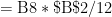
The idea is that the amount owed is multiplied by a factor $r$ (which is greater than 1), and from this product the amount paid is deducted. With this approach — and unlike the approach using calculus — the payment period would be each month and not per year. Therefore, we can write

$A_{n+1} = \displaystyle \left( 1 + \frac{0.25}{12} \right) A_n - 50$

Notice that the meaning of the 25% has changed somewhat… it’s no longer the relative rate of growth, as the 25% has been equally divided for the 12 months. The solution of this difference equation is

$A_n = r^n P - k \left( \displaystyle \frac{1 - r^n}{1-r} \right)$

A great advantage of using a difference equation to solve this problem is that the solution can be easily checked with a simple spreadsheet. (Indeed, pedagogically, I would recommend showing a spreadsheet like this before doing any of the calculations of the previous few posts, so that students can begin to wrap their heads around the notion of a difference equation before the solution is presented.)

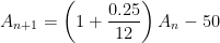
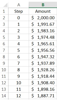
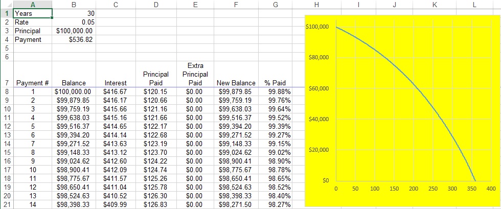
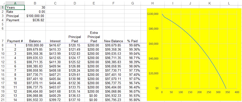
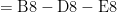
To start the spreadsheet, I wrote “Step” in Cell A1 and “Amount” in Cell B1. Then I entered the initial conditions: $0$ in Cell A2 and $2000$ in Cell B2. (In the screenshot below, I changed the format of column B to show dollars and cents.) Next, I entered $=\hbox{A2}+1$ in Cell A3 and

$=\hbox{B2}*(1+0.25/12)-50$

in Cell B3. Finally, I copied the pattern in Cells A3 and B3 downward. Here’s the result:

After the formula the algebraic solution of the difference equation has been found, this can be added to the spreadsheet in a different column. For example, I added the header “Predicted Amount” in Cell D1. In Cell D2, I typed the formula

$=2000*\hbox{POWER}(1+0.25/12,\hbox{A2})-50*(1-\hbox{POWER}(1+0.25/12,\hbox{A2}))/(1-(1+0.25/12))$

Finally, I copied this pattern down the Column D. Here’s the result:

Invariably, when I perform a demonstration like this in class, I elicit a reaction of “Whoa…. it actually works!” Even for a class of math majors. Naturally, I tease them about this… they didn’t believe me when I used algebra, but now it has to be true because the computer says so.

Here’s the spreadsheet that I used to make the above pictures: CreditCardDebt.

Exponential growth and decay (Part 7): Paying off credit-card debt via recurrence relations

You have a balance of $2,000 on your credit card. Interest is compounded continuously with a rate of growth of 25% per year. If you pay the minimum amount of $50 per month (or $600 per year), how long will it take for the balance to be paid?

$A_{n+1} = r A_n - k$

$A_{n+1} = \displaystyle \left( 1 + \frac{0.25}{12} \right) A_n - 50$

Notice that the meaning of the 25% has changed somewhat… it’s no longer the relative rate of growth, as the 25% has been equally divided for the 12 months.

A full treatment of the solution of difference equations belongs to a proper course in discrete mathematics. In the previous posts, I demonstrated how this difference equation could be solved by directly finding $A_1, A_2, A_3, \dots$ and looking for a pattern.

In this post, I’d like to present an alternative method for deriving the solution. I’ll let the reader decide for him/herself as to whether this technique is pedagogically superior to the previous method. We will attempt to find a solution of the form

$A_n = a r^n + b$ ,

where $a$ and $b$ are unknown constants.Why do we guess the solution to have this form? I won’t dive into the details, but this is entirely analogous to constructing the characteristic equation of a linear differential equation with constant coefficients as well as using the method of undetermined coefficients to find a particular solution to a inhomogeneous linear differential equation with constant coefficients.