UK Coal

Bryan Bros and Units of Measurement

For the last couple years, one of my favorite sources of entertainment has been the wonderful world of YouTube Golf. Intending no disrespect to any other content creators, my favorite channels are the ones by Grant Horvat, the Bryan Bros (not to be confused with the twin tennis duo), Peter Finch, Bryson DeChambeau (of course), and Golf Girl Games (all of them absolutely, positively should have been in the Internet Invitational… but that’s another story for another day).

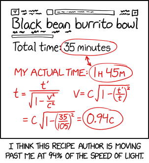
In a recent Bryan Bros video, my two interests collided. To make a long story short, a golf simulator projected that a tee shot on a par-3 ended 8 feet, 12 inches from the cup.

Co-host Wesley Bryan, to his great credit, immediately saw the computer glitch — this is an unusual way of saying the tee shot ended 9 feet from the cup. Hilarity ensued as the golfers held a stream-of-consciousness debate on the merits of metric and Imperial units. The video is below: the fun begins at the 21:41 mark and ends around 25:30.

Incoming Asteroid

Source: https://xkcd.com/3049/

Bracket Symbols

Source: https://xkcd.com/2954/

Recipe Relativity

Source: https://xkcd.com/2768/

Lagrange Points and Polynomial Equations: Index

I’m doing something that I should have done a long time ago: collecting a series of posts into one single post. The links below show my series on Lagrange points.

Part 1: Introduction

Part 2: Finding $L_1$

Part 3: Finding $L_2$

Part 4: A more analytical way of finding $L_1$ and $L_2$

Part 5: Historical anecdote: Lagrange made a careless mistake!

Musical Scales

Saturday Night Live: Washington’s Dream

Happy Fourth of July.

I’m a sucker for G-rated ways of using humor to engage students with concepts in the mathematical curriculum. I never thought that Saturday Night Live would provide a wonderful source of material for this effort.

Lagrange Points and Polynomial Equations: Part 5

This series was motivated by a terrific article that I read in the American Mathematical Monthly about Lagrange points, which are (from Wikipedia) “points of equilibrium for small-mass objects under the gravitational influence of two massive orbiting bodies.” There are five such points in the Sun-Earth system, called $L_1$ , $L_2$ , $L_3$ , $L_4$ , and $L_5$ .

The article points out a delicious historical factoid: Lagrange had a slight careless mistake in his derivation!

From the article:

Equation (d) would be just the tool to use to determine where to locate the JWST [James Webb Space Telescope, which is now in orbit about $L_2$ ], except for one thing: Lagrange got it wrong!… Do you see it? His algebra in converting $1 - \displaystyle \frac{1}{(m-1)^3}$ to common denominator form is incorrect… Fortunately, at some point in the two-and-a-half centuries between Lagrange’s work and the launch of JWST, this error has been recognized and corrected.

This little historical anecdote illustrates that, despite our best efforts, even the best of us are susceptible to careless mistakes. The simplification should have been

$q' = \displaystyle \left[ 1 - \frac{1}{(m-1)^3} \right] \cdot \frac{1}{r^3}$

$= \displaystyle \frac{(m-1)^3 - 1}{(m-1)^3} \cdot \frac{1}{r^3}$

$= \displaystyle \frac{m^3 - 3m^2 + 3m - 1 - 1}{(m-1)^3} \cdot \frac{1}{r^3}$

$= \displaystyle \frac{m^3 - 3m^2 + 3m - 2}{(m-1)^3} \cdot \frac{1}{r^3}$ .

(Parenthetically, The article also notes a clear but unintended typesetting error, as the correct but smudged exponent of 3 in the first equation became an incorrect exponent of 2 in the second.)

Lagrange Points and Polynomial Equations: Part 4

From Wikipedia, Lagrange points are points of equilibrium for small-mass objects under the gravitational influence of two massive orbiting bodies. There are five such points in the Sun-Earth system, called $L_1$ , $L_2$ , $L_3$ , $L_4$ , and $L_5$ .

The stable equilibrium points $L_4$ and $L_5$ are easiest to explain: they are the corners of equilateral triangles in the plane of Earth’s orbit. The points $L_1$ and $L_2$ are also equilibrium points, but they are unstable. Nevertheless, they have practical applications for spaceflight.

As we’ve seen, the positions of $L_1$ and $L_2$ can be found by numerically solving the fifth-order polynomial equations

$t^5 - (3-\mu) t^4 + (3-2\mu)t^3 - \mu t^2 + 2\mu t - \mu = 0$

and

$t^5 + (3-\mu) t^4 + (3-2\mu)t^3 - \mu t^2 - 2\mu t - \mu = 0$ ,

respectively. In these equations, $\mu = \displaystyle \frac{m_2}{m_1+m_2}$ where $m_1$ is the mass of the Sun and $m_2$ is the mass of Earth. Also, $t$ is the distance from the Earth to $L_1$ or $L_2$ measured as a proportion of the distance from the Sun to Earth.

We’ve also seen that, for the Sun and Earth, $mu \approx 3.00346 \times 10^{-6}$ , and numerically solving the above quintics yields $t \approx 0.000997$ for $L_1$ and $t \approx 0.01004$ for $L_2$ . In other words, $L_1$ and $L_2$ are approximately the same distance from Earth but in opposite directions.

There’s a good reason why the positive real roots of these two similar quintics are almost equal. We know that $t$ will be a lot closer to 0 than 1 because, for gravity to balance, the Lagrange points have to be a lot closer to Earth than the Sun. For this reason, the terms $\mu t^2$ and $2\mu t$ will be a lot smaller than $\mu$ , and so those two terms can be safely ignored in a first-order approximation. Also, the terms $t^5$ and $(3-\mu)t^4$ will be a lot smaller than $(3-2\mu)t^3$ , and so those two terms can also be safely ignored in a first-order approximation. Furthermore, since $\mu$ is also close to 0, the coefficient $(3-2\mu)$ can be safely replaced by just $3$ .

Consequently, the solution of both quintic equations should be close to the solution of the cubic equation

$3t^3 - \mu = 0$ ,

which is straightforward to solve:

$3t^3 = \mu$

$t^3 = \displaystyle \frac{\mu}{3}$

$t = \displaystyle \sqrt[3]{ \frac{\mu}{3} }$ .

If $\mu = 3.00346 \times 10^{-6}$ , we obtain $t \approx 0.010004$ , which is indeed reasonably close to the actual solutions for $L_1$ and $L_2$ . Indeed, this may be used as the first approximation in Newton’s method to quickly numerically evaluate the actual solutions of the two quintic polynomials.