The Incomplete Gamma and Confluent Hypergeometric Functions (Part 7)

We are finally in position to directly prove the curious integral

$\displaystyle \int_0^z t^{a-1} e^{-t} \, dt = \displaystyle e^{-z} \sum_{s=0}^\infty \frac{(a-1)!}{(a+s)!} z^{a+s}$ ,

where the right-hand side is a special case of the confluent hypergeometric function.

Step 1. Our surprising “starting” point is the combinatorical identity

$\displaystyle \sum_{s=0}^a (-1)^s \binom{n}{s} = (-1)^a \binom{n-1}{a} \qquad 0 \le a \le n-1$ ,

which we proved in the previous post.

Step 2. We now begin to manipulate this identity. Replacing $a$ with $n-a$ , we find

$\displaystyle \sum_{s=0}^{n-a} (-1)^s \binom{n}{s} = (-1)^a \binom{n-1}{n-a}$

for $0 \le n-a \le n-1$ , or $1 \le a \le n$ . Therefore,

$\displaystyle \sum_{s=0}^{n-a} (-1)^s \frac{n!}{s! (n-s)!} = \frac{(-1)^{n-a} (n-1)!}{(a-1)!(n-a)!}$

$\displaystyle \sum_{s=0}^{n-a} \frac{(-1)^s (a-1)!}{s! (n-s)!} = \frac{(-1)^{n-a}}{n \cdot (n-a)!}$

If we replace $n$ by $a+n$ , we obtain

$\displaystyle \sum_{s=0}^n \frac{(-1)^s (a-1)!}{s! (a+n-s)!} = \frac{(-1)^n}{n! (a+n)}$

for $a \ge 1$ (since we are guaranteed that $a \le a+n$ if $a \ge 1$ ).

Step 3. We now turn to the direct integration of the incomplete gamma function:

$\displaystyle \int_0^z t^{a-1} e^{-t} \, dt = \int_0^z t^{a-1} \sum_{n=0}^\infty \frac{(-t)^n}{n!} \, dt$

$= \displaystyle \sum_{n=0}^\infty \frac{(-1)^n}{n!} \int_0^z t^{a+n-1} \, dt$

$= \displaystyle \sum_{n=0}^\infty \frac{(-1)^n}{n!} \frac{z^{a+n}}{a+n}$ .

From the work in Step 2, we may substitute:

$\displaystyle \int_0^z t^{a-1} e^{-t} \, dt = \sum_{n=0}^\infty \sum_{s=0}^n \frac{(-1)^s (a-1)!}{s! (a+n-s)!} z^{a+n}$

$= \displaystyle \sum_{n=0}^\infty \sum_{s=0}^n \frac{(-1)^s}{s!} \frac{(a-1)!}{(a+n-s)!} z^{a+n}$

$= \displaystyle z^a \sum_{n=0}^\infty \sum_{s=0}^n \frac{(-1)^s z^s}{s!} \frac{(a-1)!}{(a+n-s)!} z^{n-s}$

We now use the formula for the product of two power series:

$\displaystyle \int_0^z t^{a-1} e^{-t} \, dt = \displaystyle z^a \left( \sum_{s=0}^\infty \frac{(-1)^s z^s}{s!} \right) \left( \sum_{s=0}^\infty \frac{(a-1)!}{(a+s)!} z^s \right)$

$\displaystyle = \left( \sum_{s=0}^\infty \frac{(-z)^s}{s!} \right) \left( \sum_{s=0}^\infty \frac{(a-1)!}{(a+s)!} z^{a+s} \right)$

$\displaystyle = e^{-z} \sum_{s=0}^\infty \frac{(a-1)!}{(a+s)!} z^{a+s}$

I’ll venture to say that there are several steps with this deductive derivation that look positively miraculous. However, when we were working backwards in the previous posts of this series, these miraculous steps were actually logical next steps.

And that’s the end of the direct computation of the incomplete gamma function.

The Incomplete Gamma and Confluent Hypergeometric Functions (Part 6)

In the previous posts, I showed that the curious integral

$\displaystyle \int_0^z t^{a-1} e^{-t} \, dt = \displaystyle e^{-z} \sum_{s=0}^\infty \frac{(a-1)!}{(a+s)!} z^{a+s}$ ,

where the right-hand side is a special case of the confluent hypergeometric function when $a$ is a positive integer, can be confirmed if I can show that

$\displaystyle \sum_{s=0}^a (-1)^s \binom{n}{s} = (-1)^a \binom{n-1}{a}$ ,

where $0 \le a \le n-1$ . We now prove this combinatorical identity.

Case 1. If $a=0$ , then

$\displaystyle \sum_{s=0}^0 (-1)^s \binom{n}{s} = (-1)^0 \binom{n}{0} = 1 = (-1)^0 \binom{n-1}{0}$ .

Case 2. If $1 \le a \le n-1$ , then

$\displaystyle \sum_{s=0}^a (-1)^s \binom{n}{s} = (-1)^0 \binom{n}{0} + \sum_{s=1}^{a} (-1)^s \binom{n}{s}$

$\displaystyle = 1 + \sum_{s=1}^{a} (-1)^s \binom{n}{s}$

$\displaystyle = 1 + \sum_{s=1}^a (-1)^s \left[\binom{n-1}{s-1} + \binom{n-1}{s}\right]$

$\displaystyle = 1 + \sum_{s=1}^a (-1)^s \binom{n-1}{s-1} + \sum_{s=1}^{a-1} (-1)^s \binom{n-1}{s}$

$\displaystyle = 1 + \sum_{s=0}^{a-1} (-1)^{s+1} \binom{n-1}{s} + \sum_{s=1}^a (-1)^s \binom{n-1}{s}$

$\displaystyle = 1 + (-1)^1 \binom{n-1}{0} + \sum_{s=1}^{a-1} (-1)^{s+1} \binom{n-1}{s} + \sum_{s=1}^{a-1} (-1)^s \binom{n-1}{s} + (-1)^a \binom{n-1}{a}$

$\displaystyle = 1 -1 + (-1)^a \binom{n-1}{a} + \sum_{s=1}^{a-1} (-1)^{s+1} \binom{n-1}{s} + \sum_{s=1}^{a-1} (-1)^s \binom{n-1}{s}$

$\displaystyle = (-1)^a \binom{n-1}{a} +\sum_{s=1}^{a-1} \left[(-1)^{s+1} \binom{n-1}{s} + (-1)^s \binom{n-1}{s} \right]$

$\displaystyle = (-1)^a \binom{n-1}{a} + \sum_{s=1}^{a-1} (-1)^s \binom{n-1}{s} \left[ -1 + 1 \right]$

$\displaystyle = (-1)^a \binom{n-1}{a} + \sum_{s=1}^{a-1} 0$

$\displaystyle = (-1)^a \binom{n-1}{a}$

In retrospect, I’m really surprised that I don’t remember seeing this identity before. The proof uses many of the techniques that we teach in discrete mathematics, including peeling off a term from either the start or end of a series, reindexing a sum, and the identity for constructing the terms in Pascal’s triangle in terms of the binomial coefficients. So I would’ve thought that I would’ve come across this, either in my own studies as a student or else in a textbook while preparing to teach discrete mathematics.

The observant reader may have noted that the “proof” over the past few posts isn’t really a proof since I started with the equation that I wanted to prove and then ended up with a true statement. While working backwards helped me see what was going on, this logic is ultimately flawed since it’s possible for false statements to imply true statements (another principle from discrete mathematics). I’ll clean this up in the next post.

The Incomplete Gamma and Confluent Hypergeometric Functions (Part 5)

In the previous two posts, I show that the curious integral

$\displaystyle \int_0^z t^{a-1} e^{-t} \, dt = \displaystyle e^{-z} \sum_{s=0}^\infty \frac{(a-1)!}{(a+s)!} z^{a+s}$ ,

where the right-hand side is a special case of the confluent hypergeometric function when $a$ is a positive integer, can be confirmed if I can show that

$\displaystyle \sum_{s=0}^a (-1)^s \binom{n}{s} =^? (-1)^a \binom{n-1}{a}$ .

When I first arrived at this equation, I noticed that this was really a property about the numbers in Pascal’s triangle: if we alternate adding and subtracting the binomial coefficients $\displaystyle \binom{n}{s}$ on the $n$ th row of Pascal’s triangle, the result is supposed to be an entry in the previous row (perhaps multiplied by $-1$ ).

For example, using the 10th row of Pascal’s triangle:

$1 - 10 = -9$ , which is negative the number to the “northeast” of 10.
$1 - 10 + 45 = 36$ , which is the number northeast of 45.
$1 - 10 + 45 - 120 = -84$ , which is negative the number northeast of 120.
$1 - 10 + 45 -120 + 210 = 126$ , which is the number northeast of 210.

And so on.

These computations suggest a proof of this identity. Any term in the interior of Pascal’s triangle can be found by adding the two terms immediately above it. Indeed, we can see this working out in the sequence of sums listed above.

I’ll write up the formal proof of the identity in the next post.

The Incomplete Gamma and Confluent Hypergeometric Functions (Part 4)

In the previous post, I show that the curious integral

$\displaystyle \int_0^z t^{a-1} e^{-t} \, dt = \displaystyle e^{-z} \sum_{s=0}^\infty \frac{(a-1)!}{(a+s)!} z^{a+s}$ ,

where the right-hand side is a special case of the confluent hypergeometric function when $a$ is a positive integer, can be confirmed if I can show that

$\displaystyle \sum_{s=0}^n \frac{(-1)^s (a-1)!}{s! (a+n-s)!} =^? \frac{(-1)^n}{n! (a+n)}$ .

I’m using the symbol $=^?$ to emphasize that I haven’t proven that this equality is true. To be honest, I didn’t immediately believe that this worked; however, I was psychologically convinced after using Mathematica to compute this sum for about a dozen values of $n$ and $a$ .

To attempt a proof, we first note that if $n=0$ , then

$\displaystyle \sum_{s=0}^0 \frac{(-1)^s (a-1)!}{s! (a+0-s)!} = (-1)^0 \frac{(a-1)!}{0!a!} = \frac{(-1)^0}{0! (a+0)}$ ,

and so the equality works if $n=0$ . So, for the following, we will assume that $n \ge 1$ . I tried replacing $n$ with $n-a$ in the above equation to hopefully simplify the summation a little bit:

$\displaystyle \sum_{s=0}^{n-a} \frac{(-1)^s (a-1)!}{s! (a+n-a-s)!} =^? \frac{(-1)^{n-a}}{(n-a)! (a+n-a)}$

$\displaystyle \sum_{s=0}^{n-a} \frac{(-1)^s (a-1)!}{s! (n-s)!} =^? \frac{(-1)^{n-a}}{n \cdot (n-a)!}$

$\displaystyle \sum_{s=0}^{n-a} \frac{(-1)^s}{s! (n-s)!} =^? \frac{(-1)^{n-a}}{n \cdot (a-1)!(n-a)!}$

The left-hand side looks like a binomial coefficient, which suggest multiplying both sides by $n!$ :

$\displaystyle \sum_{s=0}^{n-a} (-1)^s \frac{n!}{s! (n-s)!} =^? \frac{(-1)^{n-a} n!}{n \cdot (a-1)!(n-a)!}$

$\displaystyle \sum_{s=0}^{n-a} (-1)^s \binom{n}{s} =^? \frac{(-1)^{n-a} (n-1)!}{(a-1)!(n-a)!}$

Surprise, surprise: the right-hand side is also a binomial coefficient since $(a-1)+(n-a) = n-1$ :

$\displaystyle \sum_{s=0}^{n-a} (-1)^s \binom{n}{s} =^? (-1)^{n-a} \binom{n-1}{n-a}$ .

Now we’re getting somewhere. To again make a sum a little simpler, let’s replace $a$ with $n-a$ :

$\displaystyle \sum_{s=0}^{n-(n-a)} (-1)^s \binom{n}{s} =^? (-1)^{n-(n-a)} \binom{n-1}{n-(n-a)}$

$\displaystyle \sum_{s=0}^a (-1)^s \binom{n}{s} =^? (-1)^a \binom{n-1}{a}$

Therefore, it appears that the confirming the complicated integral at the top of this post reduces to this equality involving binomial coefficients. In the next post, I’ll directly confirm this equality.

The Incomplete Gamma and Confluent Hypergeometric Functions (Part 3)

In the previous post, I confirmed the curious integral

$\displaystyle \int_0^z t^{a-1} e^{-t} \, dt = \displaystyle e^{-z} \sum_{s=0}^\infty \frac{(a-1)!}{(a+s)!} z^{a+s}$ ,

where the right-hand side is a special case of the confluent hypergeometric function when $a$ is a positive integer, by differentiating the right-hand side. However, the confirmation psychologically felt very unsatisfactory — we basically guessed the answer and then confirmed that it worked.

A seemingly better way to approach the integral is to use the Taylor series representation of $e^{-t}$ to integrate the left-hand side term-by-term:

$\displaystyle \int_0^z t^{a-1} e^{-t} \, dt = \int_0^z t^{a-1} \sum_{n=0}^\infty \frac{(-t)^n}{n!} \, dt$

$= \displaystyle \sum_{n=0}^\infty \frac{(-1)^n}{n!} \int_0^z t^{a+n-1} \, dt$

$= \displaystyle \sum_{n=0}^\infty \frac{(-1)^n}{n!} \frac{z^{a+n}}{a+n}$ .

Well, that doesn’t look like the right-hand side of the top equation. However, the right-hand side of the top equation also has a $e^{-z}$ in it. Let’s also convert that to its Taylor series expansion and then use the formula for multiplying two infinite series:

$\displaystyle e^{-z} \sum_{s=0}^\infty \frac{(a-1)!}{(a+s)!} z^{a+s} = \left( \sum_{s=0}^\infty \frac{(-z)^s}{s!} \right) \left( \sum_{s=0}^\infty \frac{(a-1)!}{(a+s)!} z^{a+s} \right)$

$= \displaystyle z^a \left( \sum_{s=0}^\infty \frac{(-1)^s z^s}{s!} \right) \left( \sum_{s=0}^\infty \frac{(a-1)!}{(a+s)!} z^s \right)$

$= \displaystyle z^a \sum_{n=0}^\infty \sum_{s=0}^n \frac{(-1)^s z^s}{s!} \frac{(a-1)!}{(a+n-s)!} z^{n-s}$

$= \displaystyle \sum_{n=0}^\infty \sum_{s=0}^n \frac{(-1)^s}{s!} \frac{(a-1)!}{(a+n-s)!} z^{a+n}$

Summarizing, apparently the following two infinite series are supposed to be equal:

$\displaystyle \sum_{n=0}^\infty \frac{(-1)^n}{n!} \frac{z^{a+n}}{a+n} = \sum_{n=0}^\infty \sum_{s=0}^n \frac{(-1)^s}{s!} \frac{(a-1)!}{(a+n-s)!} z^{a+n}$ ,

or, matching coefficients of $z^{a+n}$ ,

$\displaystyle \frac{(-1)^n}{n! (a+n)} = \sum_{s=0}^n \frac{(-1)^s (a-1)!}{s! (a+n-s)!}$ .

When I first came to this equality, my immediate reaction was to throw up my hands and assume I made a calculation error someplace — I had a hard time believing that this sum from $s=0$ to $s=n$ was true. However, after using Mathematica to evaluate this sum for about a dozen different values of $n$ and $a$ , I was able to psychologically assure myself that this identity was somehow true.

But why does this awkward summation work? This is no longer a question about integration: it’s a question about a finite sum with factorials. I continue this exploration in the next post.

The Incomplete Gamma and Confluent Hypergeometric Functions (Part 2)

In this series of posts, I confirm this curious integral:

$\displaystyle \int_0^z t^{a-1} e^{-t} \, dt = \displaystyle \frac{z^a e^{-z}}{a} M(1, 1+a, z)$ ,

where the confluent hypergeometric function $M(a,b,z)$ is

$M(a,b,z) = \displaystyle 1+\sum_{s=1}^\infty \frac{a(a+1)\dots(a+s-1)}{b(b+1)\dots (b+s-1)} \frac{z^s}{s!}$ .

This integral can be confirmed — unsatisfactorily confirmed, but confirmed — by differentiating the right-hand side. For the sake of simplicity, I restrict my attention to the case when $a$ is a positive integer. To begin, the right-hand side is

$\displaystyle \frac{z^a e^{-z}}{a} M(1, 1+a, z) = \displaystyle \frac{z^a e^{-z}}{a} \left[1 + \sum_{s=1}^\infty \frac{1 \cdot 2 \cdot \dots \cdot s}{(a+1)(a+2)\dots (a+s)} \frac{z^s}{s!} \right]$

$= \displaystyle \frac{z^a e^{-z}}{a} \left[1 + \sum_{s=1}^\infty \frac{1}{(a+1)(a+2)\dots (a+s)} z^s \right]$

$= \displaystyle \frac{z^a e^{-z}}{a} \left[1 + \sum_{s=1}^\infty \frac{a!}{(a+s)!} z^s \right]$

$= \displaystyle \frac{z^a e^{-z}}{a} \sum_{s=0}^\infty \frac{a!}{(a+s)!} z^s$

$= \displaystyle e^{-z} \sum_{s=0}^\infty \frac{(a-1)!}{(a+s)!} z^{a+s}$ .

We now differentiate, first by using the Product Rule and then differentiating the series term-by-term (blatantly ignoring the need to confirm that term-by-term differentiation applies to this series):

$\displaystyle \frac{d}{dz} \left[\frac{z^a e^{-z}}{a} M(1, 1+a, z) \right] = \displaystyle \frac{d}{dz} \left[ e^{-z} \sum_{s=0}^\infty \frac{(a-1)!}{(a+s)!} z^{a+s} \right]$

$= -e^{-z} \displaystyle \sum_{s=0}^\infty \frac{(a-1)!}{(a+s)!} z^{a+s} + e^{-z} \frac{d}{dz} \left[ \sum_{s=0}^\infty \frac{(a-1)!}{(a+s)!} z^{a+s} \right]$

$= -e^{-z} \displaystyle \sum_{s=0}^\infty \frac{(a-1)!}{(a+s)!} z^{a+s} + e^{-z} \sum_{s=0}^\infty \frac{(a-1)!}{(a+s)!} \frac{d}{dz} z^{a+s}$

$= -e^{-z} \displaystyle \sum_{s=0}^\infty \frac{(a-1)!}{(a+s)!} z^{a+s} + e^{-z} \sum_{s=0}^\infty \frac{(a-1)!}{(a+s)!} (a+s) z^{a+s-1}$

$= -e^{-z} \displaystyle \sum_{s=0}^\infty \frac{(a-1)!}{(a+s)!} z^{a+s} + e^{-z} \sum_{s=0}^\infty \frac{(a-1)!}{(a+s-1)!} z^{a+s-1}$ .

We now shift the index of the first series:

$\displaystyle \frac{d}{dz} \left[\frac{z^a e^{-z}}{a} M(1, 1+a, z) \right] =-e^{-z} \sum_{s=1}^\infty \frac{(a-1)!}{(a+s-1)!} z^{a+s-1} + e^{-z} \sum_{s=0}^\infty \frac{(a-1)!}{(a+s-1)!} z^{a+s-1}$ .

By separating the $s=0$ term of the second series, the right-hand side becomes:

$\displaystyle -e^{-z} \sum_{s=1}^\infty \frac{(a-1)!}{(a+s-1)!} z^{a+s-1} + e^{-z} \frac{(a-1)!}{(a-1)!} z^{a-1} + e^{-z} \sum_{s=1}^\infty \frac{(a-1)!}{(a+s-1)!} z^{a+s-1}$ = e^{-z} z^{a-1}$

since the two infinite series cancel. We have thus shown that

$\displaystyle \frac{d}{dz} \left[\frac{z^a e^{-z}}{a} M(1, 1+a, z) \right] = \frac{e^{-z} z^{a-1}}{a}$ .

Therefore, we may integrate the right-hand side:

$\displaystyle \int_0^z t^{a-1} e^{-t} \, dt = \left[\frac{t^a e^{-t}}{a} M(1, 1+a, t) \right]_0^z$

$\displaystyle = \frac{z^a e^{-z}}{a} M(1, 1+a, z) - \frac{0^a e^{0}}{a} M(1, 1+a, 0)$

$\displaystyle = \frac{z^a e^{-z}}{a} M(1, 1+a, z)$ .

While this confirms the equality, this derivation still feels very unsatisfactory — we basically guessed the answer and then confirmed that it worked. In the next few posts, I’ll consider the direct verification of this series.

The Incomplete Gamma and Confluent Hypergeometric Functions (Part 1)

Yes, the title of this post is a mouthful.

While working on a research project, a trail of citations led me to this curious equality in the Digital Library of Mathematical Functions:

$\gamma(a,z) = \displaystyle \frac{z^a e^{-z}}{a} M(1, 1+a, z)$ ,

where the incomplete gamma function $\gamma(a,z)$ is

$\gamma(a,z) = \displaystyle \int_0^z t^{a-1} e^{-t} \, dt$

and the confluent hypergeometric function $M(a,b,z)$ is

$M(a,b,z) = \displaystyle 1+\sum_{s=1}^\infty \frac{a(a+1)\dots(a+s-1)}{b(b+1)\dots (b+s-1)} \frac{z^s}{s!}$ .

While I didn’t doubt that this was true — I don’t doubt this has been long established — I had an annoying problem: I didn’t really believe it. The gamma function

$\Gamma(a) = \displaystyle \int_0^\infty t^{a-1} e^{-t} \, dt$

is a well-known function with the famous property that

$\Gamma(n+1) = n!$

for non-negative integers $n$ ; this is often seen in calculus textbooks as an advanced challenge using integration by parts. The incomplete gamma function $\gamma(a,z)$ has the same look as $\Gamma(a)$ , except that the range of integration is from $0$ to $z$ (and not $\infty$ ). The gamma function appears all over the place in mathematics courses.

The confluent hypergeometric function, on the other hand, typically arises in mathematical physics as the solution of the differential equation

$z f''(z) + (b-z) f'(z) - af(z) = 0$ .

As I’m not a mathematical physicist, I won’t presume to state why this particular differential equation is important — except that it appears to be a niche equation that arises in very specialized applications.

So I had a hard time psychologically accepting that these two functions were in any way related.

While ultimately unimportant for advancing mathematics, this series will be about the journey I took to directly confirm the above equality.

Unit Circle

Source: https://xkcd.com/3041/

Solving Problems Submitted to MAA Journals: Index

I’m doing something that I should have done a long time ago: collecting a series of posts into one single post. The links below show my series on solving problems submitted to the journals of the Mathematical Association of America.

Part 1: Introduction

Part 2a: Suppose that $X$ and $Y$ are independent, uniform random variables over $[0,1]$ . Now define the random variable $Z$ by

$Z = (Y-X) {\bf 1}(Y \ge X) + (1-X+Y) {\bf 1}(Y<X)$ .

Prove that $Z$ is uniform over $[0,1]$ . Here, ${\bf 1}[S]$ is the indicator function that is equal to 1 if $S$ is true and 0 otherwise.

Part 2b: Suppose that $X$ and $Y$ are independent, uniform random variables over $[0,1]$ . Define $U_X$ , $V_X$ , $B_X$ , and $W_X$ as follows:

$U_X$ is uniform over $[0,X]$ ,

$V_X$ is uniform over $[X,1]$ ,

$B_X \in \{0,1\}$ with $P(B_X=1) = X$ and $P(B_X=0)=1-X$ , and

$W_X = B_X \cdot U_X + (1-B_X) \cdot V_X$ .

Prove that $W_X$ is uniform over $[0,1]$ .

Part 3: Define, for every non-negative integer $n$ , the $n$ th Catalan number by

$C_n := \displaystyle \frac{1}{n+1} {2n \choose n}$ .

Consider the sequence of complex polynomials in $z$ defined by $z_k := z_{k-1}^2 + z$ for every non-negative integer $k$ , where $z_0 := z$ . It is clear that $z_k$ has degree $2^k$ and thus has the representation

$z_k =\displaystyle \sum_{n=1}^{2^k} M_{n,k} z^n$ ,

where each $M_{n,k}$ is a positive integer. Prove that $M_{n,k} = C_{n-1}$ for $1 \le n \le k+1$ .

Part 4: Let $A_1, \dots, A_n$ be arbitrary events in a probability field. Denote by $B_k$ the event that at least $k$ of $A_1, \dots A_n$ occur. Prove that $\displaystyle \sum_{k=1}^n P(B_k) = \sum_{k=1}^n P(A_k)$ .

Parts 5a, 5b, 5c, 5d, and 5e: Evaluate the following sums in closed form:

$\displaystyle \sum_{n=0}^\infty \left( \cos x - 1 + \frac{x^2}{2!} - \frac{x^4}{4!} \dots + (-1)^{n-1} \frac{x^{2n}}{(2n)!} \right)$

and

$\displaystyle \sum_{n=0}^\infty \left( \sin x - x + \frac{x^3}{3!} - \frac{x^5}{5!} \dots + (-1)^{n-1} \frac{x^{2n+1}}{(2n+1)!} \right)$ .

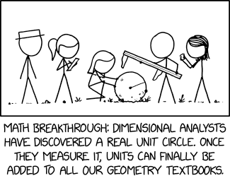
Parts 6a, 6b, 6c, 6d, and 6e: Two points $P$ and $Q$ are chosen at random (uniformly) from the interior of a unit circle. What is the probability that the circle whose diameter is segment $\overline{PQ}$ lies entirely in the interior of the unit circle?

Parts 7a, 7b, 7c, 7d, 7e, 7f, 7g, 7h, and 7i: Let $X$ and $Y$ be independent normally distributed random variables, each with its own mean and variance. Show that the variance of $X$ conditioned on the event $X>Y$ is smaller than the variance of $X$ alone.

Depressing State of STEM Graduate School Admissions

In the past couple of months, I read a couple of very sobering and depressing articles on how hard it is for talented undergraduates to be admitted into graduate school in 2026. From MAA (Mathematical Association of America) FOCUS:

Hannah’s professors kept telling her she was a shoo-in for grad school. With a published paper in symplectic geometry, another one in combinatorial game theory in the works, and a 4.0 GPA in her math classes, she was a star in her department at Rhodes College. So, when she applied to a dozen PhD programs in math with the strong support of her department, she expected to have some exciting options to weigh as acceptances rolled in. Right on schedule, her first encouraging sign came from a state school in the North. They flew her up to campus to entice her to join their program, and they offered her a nice research assistantship—but with a caveat: funding could only be guaranteed for one year. The offer sounded promising, but only one year of committed funding? That feels odd.

Not long after her campus visit, she heard back from the University of Kentucky. That’s when she really started to sense something was off. According to Hannah, Kentucky told
her, “We are currently waiting to see how things play out. You are one of the top students that we want to admit… if we can admit any students at all. Please stand by.” Her mentors validated that this was unusual, but they were confident nonetheless that more acceptances were on the way. As the April 15 deadline for students to accept offers of admission approached, Hannah heard from another school that she was on the waitlist and a couple more that she would not be receiving an offer. Oddly, she also got an Instagram message from a grad student at one of the schools she applied to. The
grad student told her, in effect, that one of the professors who was reviewing her application was so taken with her research that they were telling the other faculty and students about it. This excitement about her work gave her hope that another
offer was on the horizon—but none materialized.

And from another article from Physics Today (American Institute of Physics):

“Strange and harrowing.” That’s how Sara Earnest describes the process of applying for physics PhD programs this year. She graduated in May from Johns Hopkins University with two and a half years of undergraduate research experience. But just two weeks shy of the 15 April national deadline for prospective students to commit to graduate programs, she had been wait-listed by one, rejected by seven, and was still waiting to hear from three.

In the end, Earnest didn’t get into any of them. She plans to try again next year.

Beyond the anecdotes, the articles suggest a number of factors that have made getting into graduate school in STEM significantly harder than in past years:

Improved stipends from graduate students without additional funding from universities necessarily causes reduced cohorts.
The threat (real and perceived) of decreased federal support for STEM research: the effects on highly selective programs have a trickle-down effect on other grad programs.
After-effects of COVID and inflation.