The following problem appeared in Volume 131, Issue 9 (2024) of The American Mathematical Monthly.
Let  and
and  be independent normally distributed random variables, each with its own mean and variance. Show that the variance of conditioned on the event
  is smaller than the variance of alone.
I admit I did a double-take when I first read this problem. If and are independent, then the event contains almost no information. How then, so I thought, could the conditional distribution of given be narrower than the unconditional distribution of ?
Then I thought: I can believe that  is greater than
  : if we’re given that , then we know that must be larger than something. So maybe it’s possible for
  to be less than
  .
.
Still, not quite knowing how to start, I decided to begin by simplifying the problem and assume that both and follow a standard normal distribution, so that  and
and  . This doesn’t solve the original problem, of course, but I hoped that solving this simpler case might give me some guidance about tackling the general case. I also hoped that solving this special case might give me some psychological confidence that I would eventually be able to solve the general case.
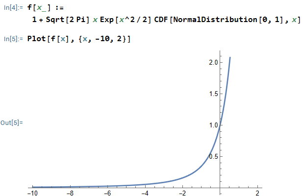
For the special case, the goal is to show that
![\hbox{Var}(X \mid X > Y) = E(X^2 \mid X > Y) - [E(X \mid X > Y)]^2 < 1](https://s0.wp.com/latex.php?latex=%5Chbox%7BVar%7D%28X+%5Cmid+X+%3E+Y%29+%3D+E%28X%5E2+%5Cmid+X+%3E+Y%29+-+%5BE%28X+%5Cmid+X+%3E+Y%29%5D%5E2+%3C+1&bg=ffffff&fg=000000&s=0&c=20201002) .
.
We begin by computing  . The denominator is straightforward: since and are independent normal random variables, we also know that
  is normally distributed with
  . (Also,
  , but that’s really not needed for this problem.) Therefore,
  since the distribution of is symmetric about its mean of
  .
.
Next,
 ,
,
where we have used the joint probability density function for and . The region of integration is  , taking care of the requirement
  . The inner integral can be directly evaluated:
![E(X I_{X>Y}) = \displaystyle \frac{1}{2\pi} \int_{-\infty}^\infty \left[ -e^{-x^2/2} \right]_x^\infty e^{-y^2/2} \, dy](https://s0.wp.com/latex.php?latex=E%28X+I_%7BX%3EY%7D%29+%3D+%5Cdisplaystyle+%5Cfrac%7B1%7D%7B2%5Cpi%7D+%5Cint_%7B-%5Cinfty%7D%5E%5Cinfty+%5Cleft%5B+-e%5E%7B-x%5E2%2F2%7D+%5Cright%5D_x%5E%5Cinfty+e%5E%7B-y%5E2%2F2%7D+%5C%2C+dy&bg=ffffff&fg=000000&s=0&c=20201002)
![= \displaystyle \frac{1}{2\pi} \int_{-\infty}^\infty \left[ 0 + e^{-y^2/2} \right] e^{-y^2/2} \, dy](https://s0.wp.com/latex.php?latex=%3D+%5Cdisplaystyle+%5Cfrac%7B1%7D%7B2%5Cpi%7D+%5Cint_%7B-%5Cinfty%7D%5E%5Cinfty+%5Cleft%5B+0+%2B+e%5E%7B-y%5E2%2F2%7D+%5Cright%5D+e%5E%7B-y%5E2%2F2%7D+%5C%2C+dy&bg=ffffff&fg=000000&s=0&c=20201002)
 .
.
At this point, I used a standard technique/trick of integration by rewriting the integrand to be the probability density function of a random variable. In this case, the random variable is normally distributed with mean 0 and variance  :
:
![E(X I_{X>Y}) = \displaystyle \frac{1}{\sqrt{2\pi} \sqrt{2}} \int_{-\infty}^\infty \frac{1}{\sqrt{2\pi} \sqrt{1/2}} \exp \left[ -\frac{y^2}{2 \cdot \frac{1}{2}} \right] \, dy](https://s0.wp.com/latex.php?latex=E%28X+I_%7BX%3EY%7D%29+%3D+%5Cdisplaystyle+%5Cfrac%7B1%7D%7B%5Csqrt%7B2%5Cpi%7D+%5Csqrt%7B2%7D%7D+%5Cint_%7B-%5Cinfty%7D%5E%5Cinfty+%5Cfrac%7B1%7D%7B%5Csqrt%7B2%5Cpi%7D+%5Csqrt%7B1%2F2%7D%7D+%5Cexp+%5Cleft%5B+-%5Cfrac%7By%5E2%7D%7B2+%5Ccdot+%5Cfrac%7B1%7D%7B2%7D%7D+%5Cright%5D+%5C%2C+dy&bg=ffffff&fg=000000&s=0&c=20201002) .
.
The integral must be equal to 1, and so we conclude
 .
.
We parenthetically note that  , matching my initial intuition.
Next, we compute the other conditional expectation:
 .
.
The inner integral can be computed using integration by parts:

![= \displaystyle \left[-x e^{-x^2/2} \right]_y^\infty + \int_y^\infty e^{-x^2/2} \, dx](https://s0.wp.com/latex.php?latex=%3D+%5Cdisplaystyle+%5Cleft%5B-x+e%5E%7B-x%5E2%2F2%7D+%5Cright%5D_y%5E%5Cinfty+%2B+%5Cint_y%5E%5Cinfty+e%5E%7B-x%5E2%2F2%7D+%5C%2C+dx&bg=ffffff&fg=000000&s=0&c=20201002)
 .
.
Therefore,

 .
.
We could calculate the first integral, but we can immediately see that it’s going to be equal to 0 since the integrand  is an odd function. The double integral is equal to
  , which we’ve already shown is equal to
  . Therefore,
  .
.
We conclude that
![\hbox{Var}(X \mid X > Y) = E(X^2 \mid X > Y) - [E(X \mid X > Y)]^2 = 1 - \displaystyle \left( \frac{1}{\sqrt{\pi}} \right)^2 = 1 - \frac{1}{\pi}](https://s0.wp.com/latex.php?latex=%5Chbox%7BVar%7D%28X+%5Cmid+X+%3E+Y%29+%3D+E%28X%5E2+%5Cmid+X+%3E+Y%29+-+%5BE%28X+%5Cmid+X+%3E+Y%29%5D%5E2+%3D+1+-+%5Cdisplaystyle+%5Cleft%28+%5Cfrac%7B1%7D%7B%5Csqrt%7B%5Cpi%7D%7D+%5Cright%29%5E2+%3D+1+-+%5Cfrac%7B1%7D%7B%5Cpi%7D&bg=ffffff&fg=000000&s=0&c=20201002) ,
,
which is indeed less than 1.
This solves the problem for the special case of two independent standard normal random variables. This of course does not yet solve the general case, but my hope was that solving this problem might give me some intuition about the general case, which I’ll develop as this series progresses.


 , then
  is always positive, where
 must be greater than
  .
.
 . If I could prove both of these claims, then that would prove that
  .
. , we integrate by parts. (This is permissible: the integrands below are well-behaved if

![= \displaystyle x e^{x^2/2} \left[ -\frac{1}{t} e^{-t^2/2} \right]_{-\infty}^x - x e^{x^2/2} \int_{-\infty}^x \frac{d}{dt} \left(\frac{1}{t} \right) \left( -e^{-t^2/2} \right) \, dt](https://s0.wp.com/latex.php?latex=%3D+%5Cdisplaystyle++x+e%5E%7Bx%5E2%2F2%7D+%5Cleft%5B+-%5Cfrac%7B1%7D%7Bt%7D+e%5E%7B-t%5E2%2F2%7D+%5Cright%5D_%7B-%5Cinfty%7D%5Ex+-+x+e%5E%7Bx%5E2%2F2%7D+%5Cint_%7B-%5Cinfty%7D%5Ex+%5Cfrac%7Bd%7D%7Bdt%7D+%5Cleft%28%5Cfrac%7B1%7D%7Bt%7D+%5Cright%29+%5Cleft%28+-e%5E%7B-t%5E2%2F2%7D+%5Cright%29+%5C%2C+dt&bg=ffffff&fg=000000&s=0&c=20201002)
![= \displaystyle x e^{x^2/2} \left[ -\frac{1}{x} e^{-x^2/2} - 0 \right] + |x| e^{x^2/2} \int_{-\infty}^x \frac{1}{t^2} e^{-t^2/2} \, dt](https://s0.wp.com/latex.php?latex=%3D+%5Cdisplaystyle++x+e%5E%7Bx%5E2%2F2%7D+%5Cleft%5B+-%5Cfrac%7B1%7D%7Bx%7D+e%5E%7B-x%5E2%2F2%7D+-+0+%5Cright%5D+%2B+%7Cx%7C+e%5E%7Bx%5E2%2F2%7D+%5Cint_%7B-%5Cinfty%7D%5Ex+%5Cfrac%7B1%7D%7Bt%5E2%7D+e%5E%7B-t%5E2%2F2%7D+%5C%2C+dt&bg=ffffff&fg=000000&s=0&c=20201002)

 .
. .
. ,
, .
. ,
, ,
,  ,
,  , and
, and  . With these definitions, we may write
  and
and  , where
  and
and  are independent standard normal random variables.
 . In previous posts, we showed that it will be sufficient to show that
  , where
  and
and  . We also showed that
  , where
  and
and
![\hbox{Var}(Z_1 \mid Z_1 > a + bZ_2) = E(Z_1^2 \mid Z_1 + a bZ_2) - [E(Z_1 \mid Z_1 > a + bZ_2)]^2](https://s0.wp.com/latex.php?latex=%5Chbox%7BVar%7D%28Z_1+%5Cmid+Z_1+%3E+a+%2B+bZ_2%29+%3D+E%28Z_1%5E2+%5Cmid+Z_1+%2B+a+bZ_2%29+-+%5BE%28Z_1+%5Cmid+Z_1+%3E+a+%2B+bZ_2%29%5D%5E2&bg=ffffff&fg=000000&s=0&c=20201002) ,
,
 .
.
![= 1 - \displaystyle\frac{c e^{-c^2/2}}{ \sqrt{2\pi} (b^2+1) \Phi(c)} - \frac{e^{-c^2}}{2\pi (b^2+1) [\Phi(c)]^2}](https://s0.wp.com/latex.php?latex=%3D+1+-++%5Cdisplaystyle%5Cfrac%7Bc+e%5E%7B-c%5E2%2F2%7D%7D%7B+%5Csqrt%7B2%5Cpi%7D+%28b%5E2%2B1%29+%5CPhi%28c%29%7D+-+%5Cfrac%7Be%5E%7B-c%5E2%7D%7D%7B2%5Cpi+%28b%5E2%2B1%29+%5B%5CPhi%28c%29%5D%5E2%7D&bg=ffffff&fg=000000&s=0&c=20201002)
![= 1 - \displaystyle\frac{c}{ \sqrt{2\pi} (b^2+1) \Phi(c) e^{c^2/2}} - \frac{1}{2\pi (b^2+1) [\Phi(c)]^2e^{c^2}}](https://s0.wp.com/latex.php?latex=%3D+1+-++%5Cdisplaystyle%5Cfrac%7Bc%7D%7B+%5Csqrt%7B2%5Cpi%7D+%28b%5E2%2B1%29+%5CPhi%28c%29+e%5E%7Bc%5E2%2F2%7D%7D+-+%5Cfrac%7B1%7D%7B2%5Cpi+%28b%5E2%2B1%29+%5B%5CPhi%28c%29%5D%5E2e%5E%7Bc%5E2%7D%7D&bg=ffffff&fg=000000&s=0&c=20201002)
![= 1 - \displaystyle\frac{\sqrt{2\pi} c e^{c^2/2} \Phi(c) + 1}{2\pi (b^2+1) [\Phi(c)]^2 e^{c^2}}](https://s0.wp.com/latex.php?latex=%3D+1+-++%5Cdisplaystyle%5Cfrac%7B%5Csqrt%7B2%5Cpi%7D+c+e%5E%7Bc%5E2%2F2%7D+%5CPhi%28c%29+%2B+1%7D%7B2%5Cpi+%28b%5E2%2B1%29+%5B%5CPhi%28c%29%5D%5E2+e%5E%7Bc%5E2%7D%7D&bg=ffffff&fg=000000&s=0&c=20201002) .
. , it suffices to show that the second term must be positive. Furthermore, since the denominator of the second term is positive, it suffices to show that
  must also be positive.
 .
. ,
, is the joint probability density function of
  .
. ,
, for the event
  .
. 
![=\displaystyle \left[ -z_1 e^{-z_1^2/2} \right]_{a+bz_2}^\infty + \int_{a+bz_2}^\infty e^{-z_1^2/2} \, dz_1](https://s0.wp.com/latex.php?latex=%3D%5Cdisplaystyle+%5Cleft%5B+-z_1+e%5E%7B-z_1%5E2%2F2%7D+%5Cright%5D_%7Ba%2Bbz_2%7D%5E%5Cinfty+%2B+%5Cint_%7Ba%2Bbz_2%7D%5E%5Cinfty+e%5E%7B-z_1%5E2%2F2%7D+%5C%2C+dz_1&bg=ffffff&fg=000000&s=0&c=20201002)
![= (a+bz_2) \displaystyle \exp \left[-\frac{(a+bz_2)^2}{2} \right] + \int_{a+bz_2}^\infty e^{-z_1^2/2} \, dz_1](https://s0.wp.com/latex.php?latex=%3D+%28a%2Bbz_2%29+%5Cdisplaystyle+%5Cexp+%5Cleft%5B-%5Cfrac%7B%28a%2Bbz_2%29%5E2%7D%7B2%7D+%5Cright%5D+%2B+%5Cint_%7Ba%2Bbz_2%7D%5E%5Cinfty+e%5E%7B-z_1%5E2%2F2%7D+%5C%2C+dz_1&bg=ffffff&fg=000000&s=0&c=20201002)
![E(Z_1^2 I_A) = \displaystyle \frac{1}{2\pi} \int_{-\infty}^\infty (a+bz_2) \exp \left[-\frac{(a+bz_2)^2}{2} \right] \exp \left[ -\frac{z_2^2}{2} \right] \, dz_2 + \int_{-\infty}^\infty \int_{a+bz_2}^\infty \frac{1}{2\pi} e^{-z_1^2/2} e^{-z_2^2/2} \, dz_1 dz_2](https://s0.wp.com/latex.php?latex=E%28Z_1%5E2+I_A%29+%3D+%5Cdisplaystyle+%5Cfrac%7B1%7D%7B2%5Cpi%7D+%5Cint_%7B-%5Cinfty%7D%5E%5Cinfty+%28a%2Bbz_2%29+%5Cexp+%5Cleft%5B-%5Cfrac%7B%28a%2Bbz_2%29%5E2%7D%7B2%7D+%5Cright%5D+%5Cexp+%5Cleft%5B+-%5Cfrac%7Bz_2%5E2%7D%7B2%7D+%5Cright%5D+%5C%2C+dz_2+%2B+%5Cint_%7B-%5Cinfty%7D%5E%5Cinfty+%5Cint_%7Ba%2Bbz_2%7D%5E%5Cinfty+%5Cfrac%7B1%7D%7B2%5Cpi%7D+e%5E%7B-z_1%5E2%2F2%7D+e%5E%7B-z_2%5E2%2F2%7D+%5C%2C+dz_1+dz_2&bg=ffffff&fg=000000&s=0&c=20201002) .
. since the double integral is
  . For the first integral, we complete the square as before:
![E(Z_1^2 I_A) = \Phi(c) + \displaystyle \frac{1}{2\pi} \int_{-\infty}^\infty (a+bz_2) \exp \left[-\frac{(b^2+1)z_2^2 + 2abz_2 + a^2}{2} \right] \, dz_2](https://s0.wp.com/latex.php?latex=E%28Z_1%5E2+I_A%29+%3D+%5CPhi%28c%29+%2B+%5Cdisplaystyle+%5Cfrac%7B1%7D%7B2%5Cpi%7D+%5Cint_%7B-%5Cinfty%7D%5E%5Cinfty+%28a%2Bbz_2%29+%5Cexp+%5Cleft%5B-%5Cfrac%7B%28b%5E2%2B1%29z_2%5E2+%2B+2abz_2+%2B+a%5E2%7D%7B2%7D+%5Cright%5D+%5C%2C+dz_2&bg=ffffff&fg=000000&s=0&c=20201002)
![= \Phi(c) + \displaystyle \frac{1}{2\pi} \int_{-\infty}^\infty (a + bz_2) \exp \left[ -\frac{b^2+1}{2} \left( z_2^2 + \frac{2abz_2}{b^2+1} \,\,\,\,\,\,\,\,\,\,\,\,\,\,\,\, \right) \right] \exp \left[ -\frac{1}{2} \left(a^2 \,\,\,\,\,\,\,\,\,\,\,\,\,\,\,\, \right) \right] dz_2](https://s0.wp.com/latex.php?latex=%3D+%5CPhi%28c%29+%2B+%5Cdisplaystyle+%5Cfrac%7B1%7D%7B2%5Cpi%7D+%5Cint_%7B-%5Cinfty%7D%5E%5Cinfty+%28a+%2B+bz_2%29+%5Cexp+%5Cleft%5B+-%5Cfrac%7Bb%5E2%2B1%7D%7B2%7D+%5Cleft%28+z_2%5E2+%2B+%5Cfrac%7B2abz_2%7D%7Bb%5E2%2B1%7D+%5C%2C%5C%2C%5C%2C%5C%2C%5C%2C%5C%2C%5C%2C%5C%2C%5C%2C%5C%2C%5C%2C%5C%2C%5C%2C%5C%2C%5C%2C%5C%2C+%5Cright%29+%5Cright%5D+%5Cexp+%5Cleft%5B+-%5Cfrac%7B1%7D%7B2%7D+%5Cleft%28a%5E2+%5C%2C%5C%2C%5C%2C%5C%2C%5C%2C%5C%2C%5C%2C%5C%2C%5C%2C%5C%2C%5C%2C%5C%2C%5C%2C%5C%2C%5C%2C%5C%2C+%5Cright%29+%5Cright%5D+dz_2&bg=ffffff&fg=000000&s=0&c=20201002)
![= \Phi(c) +\displaystyle \frac{1}{2\pi} \int_{-\infty}^\infty (a + bz_2)\exp \left[ -\frac{b^2+1}{2} \left( z_2^2 + \frac{2abz_2}{b^2+1} + \frac{a^2b^2}{(b^2+1)^2} \right) \right] \exp \left[ -\frac{1}{2} \left(a^2 - \frac{a^2b^2}{b^2+1} \right) \right] dz_2](https://s0.wp.com/latex.php?latex=%3D+%5CPhi%28c%29+%2B%5Cdisplaystyle+%5Cfrac%7B1%7D%7B2%5Cpi%7D+%5Cint_%7B-%5Cinfty%7D%5E%5Cinfty+%28a+%2B+bz_2%29%5Cexp+%5Cleft%5B+-%5Cfrac%7Bb%5E2%2B1%7D%7B2%7D+%5Cleft%28+z_2%5E2+%2B+%5Cfrac%7B2abz_2%7D%7Bb%5E2%2B1%7D+%2B+%5Cfrac%7Ba%5E2b%5E2%7D%7B%28b%5E2%2B1%29%5E2%7D+%5Cright%29+%5Cright%5D+%5Cexp+%5Cleft%5B+-%5Cfrac%7B1%7D%7B2%7D+%5Cleft%28a%5E2+-+%5Cfrac%7Ba%5E2b%5E2%7D%7Bb%5E2%2B1%7D+%5Cright%29+%5Cright%5D+dz_2&bg=ffffff&fg=000000&s=0&c=20201002)
![= \Phi(c) +\displaystyle \frac{1}{2\pi} \int_{-\infty}^\infty (a + bz_2)\exp \left[ -\frac{b^2+1}{2} \left( z_2 + \frac{ab}{b^2+1} \right)^2 \right] \exp \left[ -\frac{1}{2} \left( \frac{a^2}{b^2+1} \right) \right] dz_2](https://s0.wp.com/latex.php?latex=%3D+%5CPhi%28c%29+%2B%5Cdisplaystyle+%5Cfrac%7B1%7D%7B2%5Cpi%7D+%5Cint_%7B-%5Cinfty%7D%5E%5Cinfty+%28a+%2B+bz_2%29%5Cexp+%5Cleft%5B+-%5Cfrac%7Bb%5E2%2B1%7D%7B2%7D+%5Cleft%28+z_2+%2B+%5Cfrac%7Bab%7D%7Bb%5E2%2B1%7D+%5Cright%29%5E2+%5Cright%5D+%5Cexp+%5Cleft%5B+-%5Cfrac%7B1%7D%7B2%7D+%5Cleft%28+%5Cfrac%7Ba%5E2%7D%7Bb%5E2%2B1%7D+%5Cright%29+%5Cright%5D+dz_2&bg=ffffff&fg=000000&s=0&c=20201002)
![= \Phi(c) +\displaystyle \frac{e^{-c^2/2}}{2\pi} \int_{-\infty}^\infty (a + bz_2)\exp \left[ -\frac{b^2+1}{2} \left( z_2 + \frac{ab}{b^2+1} \right)^2 \right] dz_2](https://s0.wp.com/latex.php?latex=%3D+%5CPhi%28c%29+%2B%5Cdisplaystyle+%5Cfrac%7Be%5E%7B-c%5E2%2F2%7D%7D%7B2%5Cpi%7D+%5Cint_%7B-%5Cinfty%7D%5E%5Cinfty+%28a+%2B+bz_2%29%5Cexp+%5Cleft%5B+-%5Cfrac%7Bb%5E2%2B1%7D%7B2%7D+%5Cleft%28+z_2+%2B+%5Cfrac%7Bab%7D%7Bb%5E2%2B1%7D+%5Cright%29%5E2+%5Cright%5D+dz_2&bg=ffffff&fg=000000&s=0&c=20201002) .
. and multiplying and dividing by
  in the denominator:
![E(Z_1^2 I_A) = \Phi(c) + \displaystyle \frac{e^{-c^2/2}}{\sqrt{2\pi}\sqrt{b^2+1}} \int_{-\infty}^\infty (a+bz_2) \frac{1}{\sqrt{2\pi} \sqrt{ \displaystyle \frac{1}{b^2+1}}} \exp \left[ - \frac{\left(z_2 + \displaystyle \frac{ab}{b^2+1} \right)^2}{2 \cdot \displaystyle \frac{1}{b^2+1}} \right] dz_2](https://s0.wp.com/latex.php?latex=E%28Z_1%5E2+I_A%29+%3D+%5CPhi%28c%29+%2B+%5Cdisplaystyle+%5Cfrac%7Be%5E%7B-c%5E2%2F2%7D%7D%7B%5Csqrt%7B2%5Cpi%7D%5Csqrt%7Bb%5E2%2B1%7D%7D+%5Cint_%7B-%5Cinfty%7D%5E%5Cinfty+%28a%2Bbz_2%29+%5Cfrac%7B1%7D%7B%5Csqrt%7B2%5Cpi%7D+%5Csqrt%7B+%5Cdisplaystyle+%5Cfrac%7B1%7D%7Bb%5E2%2B1%7D%7D%7D+%5Cexp+%5Cleft%5B+-+%5Cfrac%7B%5Cleft%28z_2+%2B+%5Cdisplaystyle+%5Cfrac%7Bab%7D%7Bb%5E2%2B1%7D+%5Cright%29%5E2%7D%7B2+%5Ccdot+%5Cdisplaystyle+%5Cfrac%7B1%7D%7Bb%5E2%2B1%7D%7D+%5Cright%5D+dz_2&bg=ffffff&fg=000000&s=0&c=20201002) .
. with
with  and
and  . Therefore, the integral is equal to
  , so that
 ,
,


 .
. .
. , then
  and
and  , so that
  , matching what we found earlier.
 .
. .
. ,
, .
. ,
,![E(Z_1 I_A) = \displaystyle \frac{1}{2\pi} \int_{-\infty}^\infty \left[ - e^{-z_1^2/2} \right]_{a+bz_2}^\infty e^{-z_2^2/2} \, dz_2](https://s0.wp.com/latex.php?latex=E%28Z_1+I_A%29+%3D+%5Cdisplaystyle+%5Cfrac%7B1%7D%7B2%5Cpi%7D+%5Cint_%7B-%5Cinfty%7D%5E%5Cinfty+%5Cleft%5B+-+e%5E%7B-z_1%5E2%2F2%7D+%5Cright%5D_%7Ba%2Bbz_2%7D%5E%5Cinfty+e%5E%7B-z_2%5E2%2F2%7D+%5C%2C+dz_2+&bg=ffffff&fg=000000&s=0&c=20201002)
![= \displaystyle \frac{1}{2\pi} \int_{-\infty}^\infty \exp \left[ -\frac{(a+bz_2)^2}{2} \right] \exp\left[-\frac{z_2^2}{2} \right] dz_2](https://s0.wp.com/latex.php?latex=%3D+%5Cdisplaystyle+%5Cfrac%7B1%7D%7B2%5Cpi%7D+%5Cint_%7B-%5Cinfty%7D%5E%5Cinfty+%5Cexp+%5Cleft%5B+-%5Cfrac%7B%28a%2Bbz_2%29%5E2%7D%7B2%7D+%5Cright%5D+%5Cexp%5Cleft%5B-%5Cfrac%7Bz_2%5E2%7D%7B2%7D+%5Cright%5D+dz_2&bg=ffffff&fg=000000&s=0&c=20201002)
![= \displaystyle \frac{1}{2\pi} \int_{-\infty}^\infty \exp \left[ -\frac{(b^2+1)z_2^2+2abz_2+a^2}{2} \right]](https://s0.wp.com/latex.php?latex=%3D+%5Cdisplaystyle+%5Cfrac%7B1%7D%7B2%5Cpi%7D+%5Cint_%7B-%5Cinfty%7D%5E%5Cinfty+%5Cexp+%5Cleft%5B+-%5Cfrac%7B%28b%5E2%2B1%29z_2%5E2%2B2abz_2%2Ba%5E2%7D%7B2%7D+%5Cright%5D&bg=ffffff&fg=000000&s=0&c=20201002) .
.![E(Z_1 I_A) = \displaystyle \frac{1}{2\pi} \int_{-\infty}^\infty \exp \left[ -\frac{b^2+1}{2} \left( z_2^2 + \frac{2abz_2}{b^2+1} \,\,\,\,\,\,\,\,\,\,\,\,\,\,\,\, \right) \right] \exp \left[ -\frac{1}{2} \left(a^2 \,\,\,\,\,\,\,\,\,\,\,\,\,\,\,\, \right) \right] dz_2](https://s0.wp.com/latex.php?latex=E%28Z_1+I_A%29+%3D+%5Cdisplaystyle+%5Cfrac%7B1%7D%7B2%5Cpi%7D+%5Cint_%7B-%5Cinfty%7D%5E%5Cinfty+%5Cexp+%5Cleft%5B+-%5Cfrac%7Bb%5E2%2B1%7D%7B2%7D+%5Cleft%28+z_2%5E2+%2B+%5Cfrac%7B2abz_2%7D%7Bb%5E2%2B1%7D+%5C%2C%5C%2C%5C%2C%5C%2C%5C%2C%5C%2C%5C%2C%5C%2C%5C%2C%5C%2C%5C%2C%5C%2C%5C%2C%5C%2C%5C%2C%5C%2C+%5Cright%29+%5Cright%5D+%5Cexp+%5Cleft%5B+-%5Cfrac%7B1%7D%7B2%7D+%5Cleft%28a%5E2+%5C%2C%5C%2C%5C%2C%5C%2C%5C%2C%5C%2C%5C%2C%5C%2C%5C%2C%5C%2C%5C%2C%5C%2C%5C%2C%5C%2C%5C%2C%5C%2C+%5Cright%29+%5Cright%5D+dz_2&bg=ffffff&fg=000000&s=0&c=20201002)
![= \displaystyle \frac{1}{2\pi} \int_{-\infty}^\infty \exp \left[ -\frac{b^2+1}{2} \left( z_2^2 + \frac{2abz_2}{b^2+1} + \frac{a^2b^2}{(b^2+1)^2} \right) \right] \exp \left[ -\frac{1}{2} \left(a^2 - \frac{a^2b^2}{b^2+1} \right) \right] dz_2](https://s0.wp.com/latex.php?latex=%3D+%5Cdisplaystyle+%5Cfrac%7B1%7D%7B2%5Cpi%7D+%5Cint_%7B-%5Cinfty%7D%5E%5Cinfty+%5Cexp+%5Cleft%5B+-%5Cfrac%7Bb%5E2%2B1%7D%7B2%7D+%5Cleft%28+z_2%5E2+%2B+%5Cfrac%7B2abz_2%7D%7Bb%5E2%2B1%7D+%2B+%5Cfrac%7Ba%5E2b%5E2%7D%7B%28b%5E2%2B1%29%5E2%7D+%5Cright%29+%5Cright%5D+%5Cexp+%5Cleft%5B+-%5Cfrac%7B1%7D%7B2%7D+%5Cleft%28a%5E2+-+%5Cfrac%7Ba%5E2b%5E2%7D%7Bb%5E2%2B1%7D+%5Cright%29+%5Cright%5D+dz_2&bg=ffffff&fg=000000&s=0&c=20201002)
![= \displaystyle \frac{1}{2\pi} \int_{-\infty}^\infty \exp \left[ -\frac{b^2+1}{2} \left( z_2 + \frac{ab}{b^2+1} \right)^2 \right] \exp \left[ -\frac{1}{2} \left( \frac{a^2}{b^2+1} \right) \right] dz_2](https://s0.wp.com/latex.php?latex=%3D+%5Cdisplaystyle+%5Cfrac%7B1%7D%7B2%5Cpi%7D+%5Cint_%7B-%5Cinfty%7D%5E%5Cinfty+%5Cexp+%5Cleft%5B+-%5Cfrac%7Bb%5E2%2B1%7D%7B2%7D+%5Cleft%28+z_2+%2B+%5Cfrac%7Bab%7D%7Bb%5E2%2B1%7D+%5Cright%29%5E2+%5Cright%5D+%5Cexp+%5Cleft%5B+-%5Cfrac%7B1%7D%7B2%7D+%5Cleft%28+%5Cfrac%7Ba%5E2%7D%7Bb%5E2%2B1%7D+%5Cright%29+%5Cright%5D+dz_2&bg=ffffff&fg=000000&s=0&c=20201002)
![= \displaystyle \frac{e^{-c^2/2}}{2\pi} \int_{-\infty}^\infty \exp \left[ -\frac{b^2+1}{2} \left( z_2 + \frac{ab}{b^2+1} \right)^2 \right] dz_2](https://s0.wp.com/latex.php?latex=%3D+%5Cdisplaystyle+%5Cfrac%7Be%5E%7B-c%5E2%2F2%7D%7D%7B2%5Cpi%7D+%5Cint_%7B-%5Cinfty%7D%5E%5Cinfty+%5Cexp+%5Cleft%5B+-%5Cfrac%7Bb%5E2%2B1%7D%7B2%7D+%5Cleft%28+z_2+%2B+%5Cfrac%7Bab%7D%7Bb%5E2%2B1%7D+%5Cright%29%5E2+%5Cright%5D++dz_2&bg=ffffff&fg=000000&s=0&c=20201002) .
.![E(Z_1 I_A) = \displaystyle \frac{e^{-c^2/2}}{\sqrt{2\pi}\sqrt{b^2+1}} \int_{-\infty}^\infty \frac{1}{\sqrt{2\pi} \sqrt{ \displaystyle \frac{1}{b^2+1}}} \exp \left[ - \frac{\left(z_2 + \displaystyle \frac{ab}{b^2+1} \right)^2}{2 \cdot \displaystyle \frac{1}{b^2+1}} \right] dz_2](https://s0.wp.com/latex.php?latex=E%28Z_1+I_A%29+%3D+%5Cdisplaystyle+%5Cfrac%7Be%5E%7B-c%5E2%2F2%7D%7D%7B%5Csqrt%7B2%5Cpi%7D%5Csqrt%7Bb%5E2%2B1%7D%7D+%5Cint_%7B-%5Cinfty%7D%5E%5Cinfty++%5Cfrac%7B1%7D%7B%5Csqrt%7B2%5Cpi%7D+%5Csqrt%7B+%5Cdisplaystyle+%5Cfrac%7B1%7D%7Bb%5E2%2B1%7D%7D%7D+%5Cexp+%5Cleft%5B+-+%5Cfrac%7B%5Cleft%28z_2+%2B+%5Cdisplaystyle+%5Cfrac%7Bab%7D%7Bb%5E2%2B1%7D+%5Cright%29%5E2%7D%7B2+%5Ccdot+%5Cdisplaystyle+%5Cfrac%7B1%7D%7Bb%5E2%2B1%7D%7D+%5Cright%5D+dz_2&bg=ffffff&fg=000000&s=0&c=20201002) .
. , where
  , we have
 ,
, .
. , and
, and  , then
  , and
, and  , we have
 ,
, .
. , where
  . We begin by using the definition
![\hbox{Var}(X \mid A) = E(X^2 \mid A) - [E(X \mid A)]^2 = \displaystyle \frac{E(X^2 I_A)}{P(A)} - \left[ \frac{E(XI_A)}{P(A)} \right]^2](https://s0.wp.com/latex.php?latex=%5Chbox%7BVar%7D%28X+%5Cmid+A%29+%3D+E%28X%5E2+%5Cmid+A%29+-+%5BE%28X+%5Cmid+A%29%5D%5E2+%3D+%5Cdisplaystyle+%5Cfrac%7BE%28X%5E2+I_A%29%7D%7BP%28A%29%7D+-+%5Cleft%5B+%5Cfrac%7BE%28XI_A%29%7D%7BP%28A%29%7D+%5Cright%5D%5E2&bg=ffffff&fg=000000&s=0&c=20201002) .
. and
and  . First,
![E(XI_A) = E([\mu_1 + \sigma_1 Z_1] I_A) = \mu E(I_A) + E(\sigma_1 Z_1 I_A) = \mu_1 P(A) + \sigma_1 E(Z_1 I_A)](https://s0.wp.com/latex.php?latex=E%28XI_A%29+%3D+E%28%5B%5Cmu_1+%2B+%5Csigma_1+Z_1%5D+I_A%29+%3D+%5Cmu+E%28I_A%29+%2B+E%28%5Csigma_1+Z_1+I_A%29+%3D+%5Cmu_1+P%28A%29+%2B+%5Csigma_1+E%28Z_1+I_A%29&bg=ffffff&fg=000000&s=0&c=20201002) ,
, .
.![E(X^2 I_A) = E([\mu_1 + \sigma_1 Z_1]^2 I_A)](https://s0.wp.com/latex.php?latex=E%28X%5E2+I_A%29+%3D+E%28%5B%5Cmu_1+%2B+%5Csigma_1+Z_1%5D%5E2+I_A%29&bg=ffffff&fg=000000&s=0&c=20201002)
![= E([\mu_1^2 + 2\mu_1 \sigma_1 Z_1+ \sigma_1^2 Z_1^2] I_A)](https://s0.wp.com/latex.php?latex=%3D+E%28%5B%5Cmu_1%5E2+%2B+2%5Cmu_1+%5Csigma_1+Z_1%2B+%5Csigma_1%5E2+Z_1%5E2%5D+I_A%29&bg=ffffff&fg=000000&s=0&c=20201002)
 ,
, .
.![\hbox{Var}(A) = E(X^2 \mid A) - [ E(X \mid A) ]^2](https://s0.wp.com/latex.php?latex=%5Chbox%7BVar%7D%28A%29+%3D++E%28X%5E2+%5Cmid+A%29+-+%5B+E%28X+%5Cmid+A%29+%5D%5E2&bg=ffffff&fg=000000&s=0&c=20201002)
![= \mu_1^2 + 2 \mu_1 \sigma_1 E(Z_1 \mid A) + \sigma_1^2 E(Z_1^2 \mid A) - [\mu_1 + \sigma_1 E(Z_1 \mid A)]^2](https://s0.wp.com/latex.php?latex=%3D+%5Cmu_1%5E2+%2B+2+%5Cmu_1+%5Csigma_1+E%28Z_1+%5Cmid+A%29++%2B+%5Csigma_1%5E2+E%28Z_1%5E2+%5Cmid+A%29+-+%5B%5Cmu_1+%2B+%5Csigma_1+E%28Z_1+%5Cmid+A%29%5D%5E2&bg=ffffff&fg=000000&s=0&c=20201002)
![=\mu_1^2 + 2 \mu_1 \sigma_1 E(Z_1 \mid A) + \sigma_1^2 E(Z_1^2 \mid A) - \mu_1^2 - 2\mu_1 \sigma_1 E(Z_1 \mid A) - \sigma_1^2 [E(Z_1 \mid A)]^2](https://s0.wp.com/latex.php?latex=%3D%5Cmu_1%5E2+%2B+2+%5Cmu_1+%5Csigma_1+E%28Z_1+%5Cmid+A%29++%2B+%5Csigma_1%5E2+E%28Z_1%5E2+%5Cmid+A%29++-+%5Cmu_1%5E2+-+2%5Cmu_1+%5Csigma_1+E%28Z_1+%5Cmid+A%29+-+%5Csigma_1%5E2+%5BE%28Z_1+%5Cmid+A%29%5D%5E2&bg=ffffff&fg=000000&s=0&c=20201002)
![= \sigma_1^2 E(Z_1^2 \mid A) - [E(Z_1 \mid A)]^2](https://s0.wp.com/latex.php?latex=%3D+%5Csigma_1%5E2+E%28Z_1%5E2+%5Cmid+A%29+-+%5BE%28Z_1+%5Cmid+A%29%5D%5E2&bg=ffffff&fg=000000&s=0&c=20201002)
 .
. .
.  , where
  .
. to be arbitrary. Solving these two special cases boosted my confidence that I would eventually be able to tackle the general case, which I start to consider with this post.
![\hbox{Var}(X \mid X > Y) = E(X^2 \mid X > Y) - [E(X \mid X > Y)]^2 < \hbox{Var}(X) = \sigma_1^2](https://s0.wp.com/latex.php?latex=%5Chbox%7BVar%7D%28X+%5Cmid+X+%3E+Y%29+%3D+E%28X%5E2+%5Cmid+X+%3E+Y%29+-+%5BE%28X+%5Cmid+X+%3E+Y%29%5D%5E2+%3C+%5Chbox%7BVar%7D%28X%29+%3D+%5Csigma_1%5E2&bg=ffffff&fg=000000&s=0&c=20201002) .
. ,
,


 ,
, will also be a normal random variable with
 .
.  ,
, is the cumulative distribution function of the standard normal distribution.
 and
and  .
. and
and  , where
  could be something other than 1. The goal is to show that
 , but that’s really not needed for this problem.) Therefore,
  , where
  has a standard normal distribution. Then
 ,
, , matching the requirement
  . The inner integral can be directly evaluated:
![E(X I_{X>Y}) = \displaystyle \frac{1}{2\pi} \int_{-\infty}^\infty \left[ -e^{-x^2/2} \right]_{\sigma z}^\infty e^{-z^2/2} \, dz](https://s0.wp.com/latex.php?latex=E%28X+I_%7BX%3EY%7D%29+%3D+%5Cdisplaystyle+%5Cfrac%7B1%7D%7B2%5Cpi%7D+%5Cint_%7B-%5Cinfty%7D%5E%5Cinfty+%5Cleft%5B+-e%5E%7B-x%5E2%2F2%7D+%5Cright%5D_%7B%5Csigma+z%7D%5E%5Cinfty+e%5E%7B-z%5E2%2F2%7D+%5C%2C+dz&bg=ffffff&fg=000000&s=0&c=20201002)
![= \displaystyle \frac{1}{2\pi} \int_{-\infty}^\infty \left[ 0 + e^{-\sigma^2 z^2/2} \right] e^{-z^2/2} \, dz](https://s0.wp.com/latex.php?latex=%3D+%5Cdisplaystyle+%5Cfrac%7B1%7D%7B2%5Cpi%7D+%5Cint_%7B-%5Cinfty%7D%5E%5Cinfty+%5Cleft%5B+0+%2B+e%5E%7B-%5Csigma%5E2+z%5E2%2F2%7D+%5Cright%5D+e%5E%7B-z%5E2%2F2%7D+%5C%2C+dz&bg=ffffff&fg=000000&s=0&c=20201002)
 .
.![E(X I_{X>Y}) = \displaystyle \frac{1}{\sqrt{2\pi} \sqrt{\sigma^2+1}} \int_{-\infty}^\infty \frac{1}{\sqrt{2\pi} \sqrt{ \frac{1}{\sigma^2+1}}} \exp \left[ -\frac{z^2}{2 \cdot \frac{1}{\sigma^2+1}} \right] \, dz](https://s0.wp.com/latex.php?latex=E%28X+I_%7BX%3EY%7D%29+%3D+%5Cdisplaystyle+%5Cfrac%7B1%7D%7B%5Csqrt%7B2%5Cpi%7D+%5Csqrt%7B%5Csigma%5E2%2B1%7D%7D+%5Cint_%7B-%5Cinfty%7D%5E%5Cinfty+%5Cfrac%7B1%7D%7B%5Csqrt%7B2%5Cpi%7D+%5Csqrt%7B+%5Cfrac%7B1%7D%7B%5Csigma%5E2%2B1%7D%7D%7D+%5Cexp+%5Cleft%5B+-%5Cfrac%7Bz%5E2%7D%7B2+%5Ccdot+%5Cfrac%7B1%7D%7B%5Csigma%5E2%2B1%7D%7D+%5Cright%5D+%5C%2C+dz&bg=ffffff&fg=000000&s=0&c=20201002) .
. , and so the integral must be equal to 1. We conclude
 .
. .
.
![= \displaystyle \left[-x e^{-x^2/2} \right]_{\sigma z}^\infty + \int_{\sigma z}^\infty e^{-x^2/2} \, dx](https://s0.wp.com/latex.php?latex=%3D+%5Cdisplaystyle+%5Cleft%5B-x+e%5E%7B-x%5E2%2F2%7D+%5Cright%5D_%7B%5Csigma+z%7D%5E%5Cinfty+%2B+%5Cint_%7B%5Csigma+z%7D%5E%5Cinfty+e%5E%7B-x%5E2%2F2%7D+%5C%2C+dx&bg=ffffff&fg=000000&s=0&c=20201002)
 .
.
 .
. is an odd function. The double integral is equal to
  , which we’ve already shown is equal to
 ![\hbox{Var}(X \mid X > Y) = E(X^2 \mid X > Y) - [E(X \mid X > Y)]^2 = 1 - \displaystyle \frac{2}{\pi(\sigma^2 + 1)}](https://s0.wp.com/latex.php?latex=%5Chbox%7BVar%7D%28X+%5Cmid+X+%3E+Y%29+%3D+E%28X%5E2+%5Cmid+X+%3E+Y%29+-+%5BE%28X+%5Cmid+X+%3E+Y%29%5D%5E2+%3D+1+-+%5Cdisplaystyle+%5Cfrac%7B2%7D%7B%5Cpi%28%5Csigma%5E2+%2B+1%29%7D&bg=ffffff&fg=000000&s=0&c=20201002) ,
, , we recover the conditional variance found in the first special case.
 cannot be expressed using finitely many elementary functions. Therefore, we must resort to numerical methods instead.


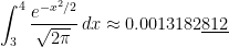

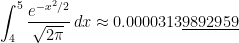


 subintervals provides a better approximation to
  than the normalcdf function.