I’m doing something that I should have done a long time ago: collecting a series of posts into one single post. The links below show my series on solving problems submitted to the journals of the Mathematical Association of America.
Part 1: Introduction
Part 2a: Suppose that  and
and  are independent, uniform random variables over
 ![[0,1]](https://s0.wp.com/latex.php?latex=%5B0%2C1%5D&bg=ffffff&fg=000000&s=0&c=20201002) . Now define the random variable
. Now define the random variable  by
by
 .
.
Prove that is uniform over . Here, ![{\bf 1}[S]](https://s0.wp.com/latex.php?latex=%7B%5Cbf+1%7D%5BS%5D&bg=ffffff&fg=000000&s=0&c=20201002) is the indicator function that is equal to 1 if
is the indicator function that is equal to 1 if  is true and 0 otherwise.
Part 2b: Suppose that and are independent, uniform random variables over . Define  ,
,  ,
,  , and
, and  as follows:
is uniform over ![[0,X]](https://s0.wp.com/latex.php?latex=%5B0%2CX%5D&bg=ffffff&fg=000000&s=0&c=20201002) ,
,
is uniform over ![[X,1]](https://s0.wp.com/latex.php?latex=%5BX%2C1%5D&bg=ffffff&fg=000000&s=0&c=20201002) ,
,
 with
with  and
and  , and
, and
 .
.
Prove that is uniform over .
Part 3: Define, for every non-negative integer  , the th Catalan number by
 .
.
Consider the sequence of complex polynomials in  defined by
  for every non-negative integer
  , where
  . It is clear that
  has degree
  and thus has the representation
 ,
,
where each  is a positive integer. Prove that
  for
for  .
.
Part 4: Let  be arbitrary events in a probability field. Denote by
  the event that at least of
  occur. Prove that
  .
.
Parts 5a, 5b, 5c, 5d, and 5e: Evaluate the following sums in closed form:

and
 .
.
Parts 6a, 6b, 6c, 6d, and 6e: Two points  and
and  are chosen at random (uniformly) from the interior of a unit circle. What is the probability that the circle whose diameter is segment
  lies entirely in the interior of the unit circle?
Parts 7a, 7b, 7c, 7d, 7e, 7f, 7g, 7h, and 7i: Let and be independent normally distributed random variables, each with its own mean and variance. Show that the variance of conditioned on the event  is smaller than the variance of alone.
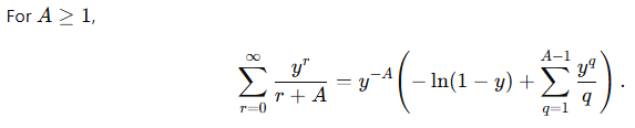


![\displaystyle \sum_{r=0}^\infty \frac{y^{r}}{r+A} = \frac{1}{y^A} \left[ -\ln(1-y) - \sum_{q=1}^{A-1} \frac{y^q}{q} \right]](https://s0.wp.com/latex.php?latex=%5Cdisplaystyle+%5Csum_%7Br%3D0%7D%5E%5Cinfty+%5Cfrac%7By%5E%7Br%7D%7D%7Br%2BA%7D+%3D+%5Cfrac%7B1%7D%7By%5EA%7D+%5Cleft%5B+-%5Cln%281-y%29+-+%5Csum_%7Bq%3D1%7D%5E%7BA-1%7D+%5Cfrac%7By%5Eq%7D%7Bq%7D+%5Cright%5D&bg=ffffff&fg=000000&s=0&c=20201002)

 ,
, ,
, with
with  , we find
 , or
, or  . Therefore,

 , we obtain
 (since we are guaranteed that
  if
if 

 .
.


 ,
, . We now prove this combinatorical identity.
 , then
  .
. , then

![\displaystyle = 1 + \sum_{s=1}^a (-1)^s \left[\binom{n-1}{s-1} + \binom{n-1}{s}\right]](https://s0.wp.com/latex.php?latex=%5Cdisplaystyle+%3D+1++%2B+%5Csum_%7Bs%3D1%7D%5Ea+%28-1%29%5Es+%5Cleft%5B%5Cbinom%7Bn-1%7D%7Bs-1%7D+%2B+%5Cbinom%7Bn-1%7D%7Bs%7D%5Cright%5D+&bg=ffffff&fg=000000&s=0&c=20201002)


![\displaystyle = (-1)^a \binom{n-1}{a} +\sum_{s=1}^{a-1} \left[(-1)^{s+1} \binom{n-1}{s} + (-1)^s \binom{n-1}{s} \right]](https://s0.wp.com/latex.php?latex=%5Cdisplaystyle+%3D+%28-1%29%5Ea+%5Cbinom%7Bn-1%7D%7Ba%7D+%2B%5Csum_%7Bs%3D1%7D%5E%7Ba-1%7D+%5Cleft%5B%28-1%29%5E%7Bs%2B1%7D+%5Cbinom%7Bn-1%7D%7Bs%7D+%2B+%28-1%29%5Es+%5Cbinom%7Bn-1%7D%7Bs%7D+%5Cright%5D&bg=ffffff&fg=000000&s=0&c=20201002)
![\displaystyle = (-1)^a \binom{n-1}{a} + \sum_{s=1}^{a-1} (-1)^s \binom{n-1}{s} \left[ -1 + 1 \right]](https://s0.wp.com/latex.php?latex=%5Cdisplaystyle+%3D+%28-1%29%5Ea+%5Cbinom%7Bn-1%7D%7Ba%7D+%2B+%5Csum_%7Bs%3D1%7D%5E%7Ba-1%7D+%28-1%29%5Es+%5Cbinom%7Bn-1%7D%7Bs%7D+%5Cleft%5B+-1+%2B+1+%5Cright%5D&bg=ffffff&fg=000000&s=0&c=20201002)


 .
. on the
  ).
).
 , which is negative the number to the “northeast” of 10.
  , which is the number northeast of 45.
 , which is negative the number northeast of 120.
 , which is the number northeast of 210.
  .
. to emphasize that I haven’t proven that this equality is true. To be honest, I didn’t immediately believe that this worked; however, I was psychologically convinced after using Mathematica to compute this sum for about a dozen values of
  , then
 ,
, . I tried replacing


 :
:

 :
: .
.
 to integrate the left-hand side term-by-term:
 in it. Let’s also convert that to its Taylor series expansion and then use the formula for multiplying two infinite series:

 ,
, ,
, .
. to
to  was true. However, after using Mathematica to evaluate this sum for about a dozen different values of
  ,
, is
is .
.![\displaystyle \frac{z^a e^{-z}}{a} M(1, 1+a, z) = \displaystyle \frac{z^a e^{-z}}{a} \left[1 + \sum_{s=1}^\infty \frac{1 \cdot 2 \cdot \dots \cdot s}{(a+1)(a+2)\dots (a+s)} \frac{z^s}{s!} \right]](https://s0.wp.com/latex.php?latex=%5Cdisplaystyle+%5Cfrac%7Bz%5Ea+e%5E%7B-z%7D%7D%7Ba%7D+M%281%2C+1%2Ba%2C+z%29+%3D+%5Cdisplaystyle+%5Cfrac%7Bz%5Ea+e%5E%7B-z%7D%7D%7Ba%7D+%5Cleft%5B1+%2B+%5Csum_%7Bs%3D1%7D%5E%5Cinfty+%5Cfrac%7B1+%5Ccdot+2+%5Ccdot+%5Cdots+%5Ccdot+s%7D%7B%28a%2B1%29%28a%2B2%29%5Cdots+%28a%2Bs%29%7D+%5Cfrac%7Bz%5Es%7D%7Bs%21%7D+%5Cright%5D&bg=ffffff&fg=000000&s=0&c=20201002)
![= \displaystyle \frac{z^a e^{-z}}{a} \left[1 + \sum_{s=1}^\infty \frac{1}{(a+1)(a+2)\dots (a+s)} z^s \right]](https://s0.wp.com/latex.php?latex=%3D+%5Cdisplaystyle+%5Cfrac%7Bz%5Ea+e%5E%7B-z%7D%7D%7Ba%7D+%5Cleft%5B1+%2B+%5Csum_%7Bs%3D1%7D%5E%5Cinfty+%5Cfrac%7B1%7D%7B%28a%2B1%29%28a%2B2%29%5Cdots+%28a%2Bs%29%7D+z%5Es+%5Cright%5D&bg=ffffff&fg=000000&s=0&c=20201002)
![= \displaystyle \frac{z^a e^{-z}}{a} \left[1 + \sum_{s=1}^\infty \frac{a!}{(a+s)!} z^s \right]](https://s0.wp.com/latex.php?latex=%3D+%5Cdisplaystyle+%5Cfrac%7Bz%5Ea+e%5E%7B-z%7D%7D%7Ba%7D+%5Cleft%5B1+%2B+%5Csum_%7Bs%3D1%7D%5E%5Cinfty+%5Cfrac%7Ba%21%7D%7B%28a%2Bs%29%21%7D+z%5Es+%5Cright%5D&bg=ffffff&fg=000000&s=0&c=20201002)

 .
.![\displaystyle \frac{d}{dz} \left[\frac{z^a e^{-z}}{a} M(1, 1+a, z) \right] = \displaystyle \frac{d}{dz} \left[ e^{-z} \sum_{s=0}^\infty \frac{(a-1)!}{(a+s)!} z^{a+s} \right]](https://s0.wp.com/latex.php?latex=%5Cdisplaystyle+%5Cfrac%7Bd%7D%7Bdz%7D+%5Cleft%5B%5Cfrac%7Bz%5Ea+e%5E%7B-z%7D%7D%7Ba%7D+M%281%2C+1%2Ba%2C+z%29+%5Cright%5D+%3D+%5Cdisplaystyle+%5Cfrac%7Bd%7D%7Bdz%7D+%5Cleft%5B+e%5E%7B-z%7D+%5Csum_%7Bs%3D0%7D%5E%5Cinfty+%5Cfrac%7B%28a-1%29%21%7D%7B%28a%2Bs%29%21%7D+z%5E%7Ba%2Bs%7D+%5Cright%5D&bg=ffffff&fg=000000&s=0&c=20201002)
![= -e^{-z} \displaystyle \sum_{s=0}^\infty \frac{(a-1)!}{(a+s)!} z^{a+s} + e^{-z} \frac{d}{dz} \left[ \sum_{s=0}^\infty \frac{(a-1)!}{(a+s)!} z^{a+s} \right]](https://s0.wp.com/latex.php?latex=%3D+-e%5E%7B-z%7D+%5Cdisplaystyle+%5Csum_%7Bs%3D0%7D%5E%5Cinfty+%5Cfrac%7B%28a-1%29%21%7D%7B%28a%2Bs%29%21%7D+z%5E%7Ba%2Bs%7D+%2B+e%5E%7B-z%7D+%5Cfrac%7Bd%7D%7Bdz%7D+%5Cleft%5B++%5Csum_%7Bs%3D0%7D%5E%5Cinfty+%5Cfrac%7B%28a-1%29%21%7D%7B%28a%2Bs%29%21%7D+z%5E%7Ba%2Bs%7D+%5Cright%5D&bg=ffffff&fg=000000&s=0&c=20201002)


 .
.![\displaystyle \frac{d}{dz} \left[\frac{z^a e^{-z}}{a} M(1, 1+a, z) \right] =-e^{-z} \sum_{s=1}^\infty \frac{(a-1)!}{(a+s-1)!} z^{a+s-1} + e^{-z} \sum_{s=0}^\infty \frac{(a-1)!}{(a+s-1)!} z^{a+s-1}](https://s0.wp.com/latex.php?latex=%5Cdisplaystyle+%5Cfrac%7Bd%7D%7Bdz%7D+%5Cleft%5B%5Cfrac%7Bz%5Ea+e%5E%7B-z%7D%7D%7Ba%7D+M%281%2C+1%2Ba%2C+z%29+%5Cright%5D+%3D-e%5E%7B-z%7D+%5Csum_%7Bs%3D1%7D%5E%5Cinfty+%5Cfrac%7B%28a-1%29%21%7D%7B%28a%2Bs-1%29%21%7D+z%5E%7Ba%2Bs-1%7D+%2B+e%5E%7B-z%7D+%5Csum_%7Bs%3D0%7D%5E%5Cinfty+%5Cfrac%7B%28a-1%29%21%7D%7B%28a%2Bs-1%29%21%7D+z%5E%7Ba%2Bs-1%7D&bg=ffffff&fg=000000&s=0&c=20201002) .
. = e^{-z} z^{a-1}$
![\displaystyle \frac{d}{dz} \left[\frac{z^a e^{-z}}{a} M(1, 1+a, z) \right] = \frac{e^{-z} z^{a-1}}{a}](https://s0.wp.com/latex.php?latex=%5Cdisplaystyle+%5Cfrac%7Bd%7D%7Bdz%7D+%5Cleft%5B%5Cfrac%7Bz%5Ea+e%5E%7B-z%7D%7D%7Ba%7D+M%281%2C+1%2Ba%2C+z%29+%5Cright%5D+%3D+%5Cfrac%7Be%5E%7B-z%7D+z%5E%7Ba-1%7D%7D%7Ba%7D&bg=ffffff&fg=000000&s=0&c=20201002) .
.![\displaystyle \int_0^z t^{a-1} e^{-t} \, dt = \left[\frac{t^a e^{-t}}{a} M(1, 1+a, t) \right]_0^z](https://s0.wp.com/latex.php?latex=%5Cdisplaystyle+%5Cint_0%5Ez+t%5E%7Ba-1%7D+e%5E%7B-t%7D+%5C%2C+dt+%3D+%5Cleft%5B%5Cfrac%7Bt%5Ea+e%5E%7B-t%7D%7D%7Ba%7D+M%281%2C+1%2Ba%2C+t%29+%5Cright%5D_0%5Ez&bg=ffffff&fg=000000&s=0&c=20201002)

 .
. ,
, is
is


 , except that the range of integration is from
  to
to  ). The gamma function appears all over the place in mathematics courses.
 .
. ,
, is a positive integer. If we perform the substitution
  in the above integral, where
  is a quantity independent of
  , we obtain
 ,
,

 and
and  in the above gamma equation, and using the fact that
  , we obtain

![I = \displaystyle \int_0^\infty -\left[ \frac{e^{-xt} (\cos x + t \sin x)}{1+t^2} \right]_{x=0}^{x=\infty} \, dt](https://s0.wp.com/latex.php?latex=I+%3D+%5Cdisplaystyle+%5Cint_0%5E%5Cinfty+-%5Cleft%5B+%5Cfrac%7Be%5E%7B-xt%7D+%28%5Ccos+x+%2B+t+%5Csin+x%29%7D%7B1%2Bt%5E2%7D+%5Cright%5D_%7Bx%3D0%7D%5E%7Bx%3D%5Cinfty%7D+%5C%2C+dt&bg=ffffff&fg=000000&s=0&c=20201002)
![= \displaystyle \int_0^\infty \left[0 +\frac{e^{0} (\cos 0 + t \sin 0)}{1+t^2} \right] \, dt](https://s0.wp.com/latex.php?latex=%3D+%5Cdisplaystyle+%5Cint_0%5E%5Cinfty+%5Cleft%5B0+%2B%5Cfrac%7Be%5E%7B0%7D+%28%5Ccos+0+%2B+t+%5Csin+0%29%7D%7B1%2Bt%5E2%7D+%5Cright%5D+%5C%2C+dt&bg=ffffff&fg=000000&s=0&c=20201002)
 .
.![I = \displaystyle \left[ \tan^{-1} t \right]_0^\infty = \displaystyle \frac{\pi}{2} - 0 = \displaystyle \frac{\pi}{2}](https://s0.wp.com/latex.php?latex=I+%3D+%5Cdisplaystyle+%5Cleft%5B+%5Ctan%5E%7B-1%7D+t+%5Cright%5D_0%5E%5Cinfty+%3D+%5Cdisplaystyle+%5Cfrac%7B%5Cpi%7D%7B2%7D+-+0+%3D+%5Cdisplaystyle+%5Cfrac%7B%5Cpi%7D%7B2%7D&bg=ffffff&fg=000000&s=0&c=20201002) .
.