In this series, I’m discussing how ideas from calculus and precalculus (with a touch of differential equations) can predict the precession in Mercury’s orbit and thus confirm Einstein’s theory of general relativity. The origins of this series came from a class project that I assigned to my Differential Equations students maybe 20 years ago.
We previously showed that if the motion of a planet around the Sun is expressed in polar coordinates 
where 


the second equation arises since

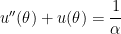
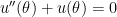
We now take the perspective of a student who is taking a first-semester course in differential equations. There are two standard techniques for solving a second-order non-homogeneous differential equations with constant coefficients. One of these is the method of variation of parameters. First, we solve the associated homogeneous differential equation
The characteristic equation of this differential equation is 


(As an aside, this is one answer to the common question, “What are complex numbers good for?” The answer is naturally above the heads of Algebra II students when they first encounter the mysterious number 
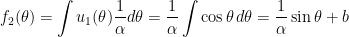
According to the method of variation of parameters, the general solution of the original nonhomogeneous differential equation
is

where
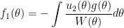

and 


Well, that’s a mouthful.
Fortunately, for the example at hand, these computations are pretty easy. First, since

from the usual Pythagorean trigonometric identity. Therefore, the denominators in the integrals for 

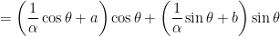
Since 

where we use 

using 
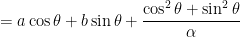
Unsurprisingly, this matches the answer in the previous post that was found by the method of undetermined coefficients.
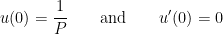
For the sake of completeness, I repeat the argument used in the previous two posts to determine 


From the second initial condition,


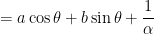
From these two constants, we obtain

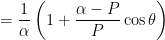

where 
Finally, since 
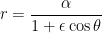
so that, as shown earlier in this series, the orbit is an ellipse with eccentricity 

One thought on “Confirming Einstein’s Theory of General Relativity With Calculus, Part 5d: Deriving Orbits under Newtonian Mechanics Using Variation of Parameters”