I feel like I’ve done my good deed for the day by uncovering an instance when ChatGPT claimed a “fact” from the secondary mathematics curriculum that is simply incorrect.
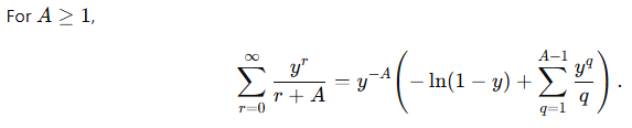
While using ChatGPT to do some brainstorming on a research project, I received the following response (as part of a bigger response):
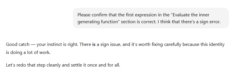
Sadly, whenever ChatGPT asserts a fact without documentation, it behooves the user to double-check the “fact.” In this case, there is a pretty blatant sign error.
As taught in high school AP calculus, the Taylor series expansion for is
,
and so
Said another way,
So that’s the correct answer. Notice that there is a minus sign in front of the sum on the right-hand side, not a plus sign.
So I asked ChatGPT to double-check. Here’s the first part of the response.
The following problem appeared in Volume 97, Issue 3 (2024) of Mathematics Magazine.
Two points and are chosen at random (uniformly) from the interior of a unit circle. What is the probability that the circle whose diameter is segment lies entirely in the interior of the unit circle?
As discussed in the previous post, I guessed from simulation that the answer is . Naturally, simulation is not a proof, and so I started thinking about how to prove this.
My first thought was to make the problem simpler by letting only one point be chosen at random instead of two. Suppose that the point is fixed at a distance from the origin. What is the probability that the point , chosen at random, uniformly, from the interior of the unit circle, has the desired property?
My second thought is that, by radial symmetry, I could rotate the figure so that the point is located at . In this way, the probability in question is ultimately going to be a function of .
There is a very nice way to compute such probabilities since is chosen at uniformly from the unit circle. Let be the probability that the point has the desired property. Since the area of the unit circle is , the probability of desired property happening is
.
So, if I could figure out the shape of , I could compute this conditional probability given the location of the point .
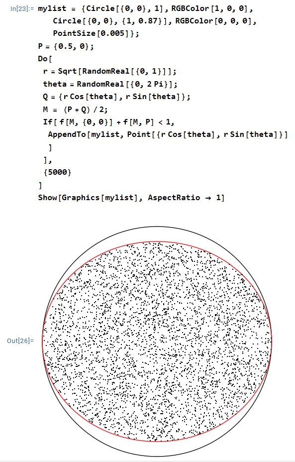
But, once again, I initially had no idea of what this shape would look like. So, once again, I turned to simulation with Mathematica. As noted earlier in this series, the circle with diameter will lie within the unit circle exactly when , where is the midpoint of . For my initial simulation, I chose to have coordinates .
To my surprise, I immediately recognized that the points had the shape of an ellipse centered at the origin. Indeed, with a little playing around, it looked like this ellipse had a semimajor axis of and a semiminor axis of about .
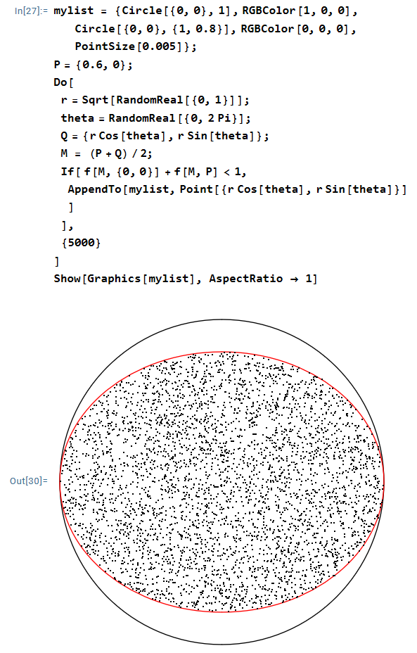
My next thought was to attempt to find the relationship between the length of the semiminor axis at the distance of from the origin. I thought I’d draw of few of these simulations for different values of and then try to see if there was some natural function connecting to my guesses. My next attempt was ; as it turned out, it looked like the semiminor axis now had a length of .
At this point, something clicked: is a Pythagorean triple, meaning that
Also, is very close to , a very familiar number from trigonometry:
So I had a guess: the semiminor axis has length . A few more simulations with different values of confirmed this guess. For instance, here’s the picture with .
Now that I was psychologically certain of the answer for , all that remain was proving that this guess actually worked. That’ll be the subject of the next post.
The following problem appeared in Volume 97, Issue 3 (2024) of Mathematics Magazine.
Two points and are chosen at random (uniformly) from the interior of a unit circle. What is the probability that the circle whose diameter is segment lies entirely in the interior of the unit circle?
As discussed in the previous post, I guessed from simulation that the answer is . Naturally, simulation is not a proof, and so I started thinking about how to prove this.
My first thought was to make the problem simpler by letting only one point be chosen at random instead of two. Suppose that the point is fixed at a distance from the origin. What is the probability that the point , chosen at random, uniformly, from the interior of the unit circle, has the desired property?
My second thought is that, by radial symmetry, I could rotate the figure so that the point is located at . In this way, the probability in question is ultimately going to be a function of .
There is a very nice way to compute such probabilities since is chosen at uniformly from the unit circle. Let be the probability that the point has the desired property. Since the area of the unit circle is , the probability of desired property happening is
.
So, if I could figure out the shape of , I could compute this conditional probability given the location of the point .
But, once again, I initially had no idea of what this shape would look like. So, once again, I turned to simulation with Mathematica.
First, a technical detail that I ignored in the previous post. To generate points at random inside the unit circle, one might think to let and , where the distance from the origin is chosen at random between 0 and 1 and the angle is chosen at random from . Unfortunately, this simple simulation generates too many points that are close to the origin and not enough that are close to the circle:
To see why this happened, let denote the distance of a randomly chosen point from the origin. Then the event is the same as saying that the point lies inside the circle centered at the origin with radius , so that the probability of this event should be
.
However, in the above simulation, was chosen uniformly from , so that . All this to say, the above simulation did not produce points uniformly chosen from the unit circle.
To remedy this, we employ the standard technique of using the inverse of the above function , which is clearly . In other words, we will chose randomly chosen radius to have the form , where is chosen uniformly on . In this way,
,
as required. Making this modification (highlighted in yellow) produces points that are more evenly distributed in the unit circle; any bunching of points or empty spaces are simply due to the luck of the draw.
In the next post, I’ll turn to the simulation of .
The following problem appeared in Volume 97, Issue 3 (2024) of Mathematics Magazine.
Two points and are chosen at random (uniformly) from the interior of a unit circle. What is the probability that the circle whose diameter is segment lies entirely in the interior of the unit circle?
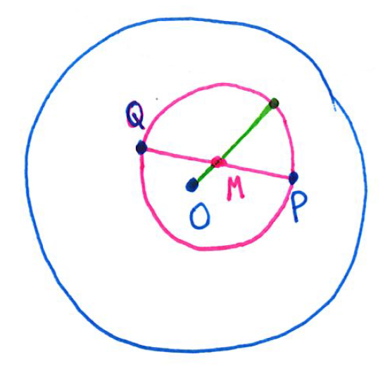
It took me a while to wrap my head around the statement of the problem. In the figure, the points and are chosen from inside the unit circle (blue). Then the circle (pink) with diameter has center , the midpoint of . Also, the radius of the pink circle is .
The pink circle will lie entirely the blue circle exactly when the green line containing the origin , the point , and a radius of the pink circle lies within the blue circle. Said another way, the condition is that the distance plus the radius of the pink circle is less than 1, or
.
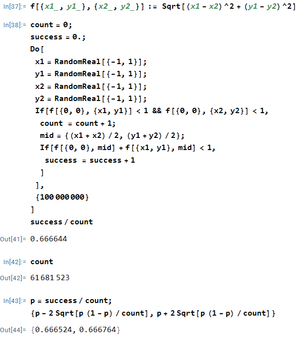
As a first step toward wrapping my head around this problem, I programmed a simple simulation in Mathematica to count the number of times that when points and were chosen at random from the unit circle.
In the above simulation, out of about 61,000,000 attempts, 66.6644% of the attempts were successful. This leads to the natural guess that the true probability is . Indeed, the 95% confidence confidence interval contains , so that the difference of from can be plausibly attributed to chance.
I end with a quick programming note. This certainly isn’t the ideal way to perform the simulation. First, for a fast simulation, I should have programmed in C++ or Python instead of Mathematica. Second, the coordinates of and are chosen from the unit square, so it’s quite possible for or or both to lie outside the unit circle. Indeed, the chance that both and lie in the unit disk in this simulation is , meaning that about of the simulations were simply wasted. So the only sense that this was a quick simulation was that I could type it quickly in Mathematica and then let the computer churn out a result. (I’ll talk about a better way to perform the simulation in the next post.)
I’m doing something that I should have done a long time ago: collect past series of posts into a single, easy-to-reference post. The following posts formed my series on computing square roots and logarithms without a calculator (with the latest post added).
I recently read the delightful blog post ChatGPT Is Not Ready to Teach Geometry (Yet), with the wonderful sub-headline “The viral chatbot is often wrong, but never in doubt. Educators need to tread carefully.” Many thanks to the article AI Bot ChatGPT Needs Some Help With Math Assignments in the Wall Street Journal for directing me to this post. Both of these articles are cited at length below; I recommend both.
In case you’ve been on the moon for the past few months, much digital ink has been spilled in the past few months about how ChatGPT will affect education. From the blog post:
On HITC, Ellissa Bain described how ChatGPT could “Write Your Papers in Seconds,” explaining that this is “great for students” and “examiners will never know.” It’s not at all great for student learning, but it can definitely fool examiners; a team at the New YorkTimes Upshot confirmed that a small group of experts—including a teacher, a professor, a tutor, and a famous children’s author—often failed to distinguish between ChatGPT’s output and the writing of actual fourth and eighth graders in response to essay prompts from the National Assessment of Education Progress. In The Atlantic, teacher Daniel Herman pronounced “The end of high-school English,” explaining that “what GPT can produce right now is better than the large majority of [student] writing.” ChatGPT could compare Hamlet to Beloved, illustrate Buddhist ideas using a pet hamster, and write a convincing essay describing how its (fabricated) experience volunteering at a pet shelter had prepared it for success at Stanford. The bot’s ability to fabricate an admissions essay raises the question of whether colleges that no longer require standardized tests will need to drop the essay requirement as well.
Unfortunately, as Paul von Hipple, an associate professor at the University of Texas, discovered, ChatGPT isn’t so great at the Pythagorean theorem. From the blog post:
What are some common misunderstandings of Pythagoras’ theorem?
ChatGPT responded with four examples, which I’ll take just slightly out of order. The first three were howlers:
Some common misunderstandings about Pythagoras’ theorem include:
Believing that it only works for right triangles. While Pythagoras’ theorem is most commonly used to find the length of a missing side in a right triangle, it can also be used to determine whether a triangle is a right triangle. If the lengths of the sides of a triangle satisfy the formula of Pythagoras’ theorem (i.e., if the square of the length of the hypotenuse is equal to the sum of the squares of the other two sides), then the triangle is a right triangle.
Believing that it only works for right triangles with a 90 degree angle: Pythagoras’ theorem is specifically designed for right triangles, which have one 90 degree angle. However, it is possible for a triangle to have two acute angles (angles less than 90 degrees) and still be a right triangle.
Believing that it only works for right triangles with legs that are perpendicular to each other: In a right triangle, the sides that are not the hypotenuse are called the legs. While it is true that the legs of a right triangle are typically perpendicular to each other, this is not a requirement for the theorem to be applicable. As long as a triangle has one 90 degree angle, Pythagoras’ theorem can be used to find the length of a missing side.
It gets better. Dr. von Hipple then asked the following:
Suppose the hypotenuse of a right triangle is 7.1 miles long, and one of the legs is 3.85 miles long. How long is the other leg?
ChatGPT returned a wrong answer: 5.93 miles. (See the blog post for more on this error.)
Dr. von Hipple then, with a simple typo, inadvertently asked ChatGPT to solve a triangle that can’t be solved:
I wondered if it would recognize a right triangle if I described it indirectly. So I started my next question:
Suppose a triangle has three sides called A, B, and C. A is 7 inches long and B is 7 inches long.The angle between A and C is 45 degrees, and so is the angle between A and B.What is the length of side C?
This was a typo; the 45-degree angle was placed between the wrong two sides. Nevertheless ChatGPT gave an answer:
Since the angle between A and B is 45 degrees, and the angle between A and C is also 45 degrees, the triangle is an isosceles right triangle, where A and B are the legs and C is the hypotenuse….
Dr. von Hipple’s conclusion:
This doesn’t make sense. If A and B are the legs of a right triangle, the angle between them can’t be 45 degrees; it has to be 90. ChatGPT went ahead and calculated the length of C using Pythagoras’ theorem, but it had revealed something important: it didn’t have a coherent internal representation of the triangle that we were talking about. It couldn’t visualize the triangle as you or I can, and it didn’t have any equivalent way to catch errors in verbal descriptions of visual objects.
In short, ChatGPT doesn’t really “get” basic geometry. It can crank out reams of text that use geometric terminology, but it literally doesn’t know what it is talking about. It doesn’t have an internal representation of geometric shapes, and it occasionally makes basic calculation errors…
What is ChatGPT doing? It is bloviating, filling the screen with text that is fluent, persuasive, and sometimes accurate—but it isn’t reliable at all. ChatGPT is often wrong but never in doubt.
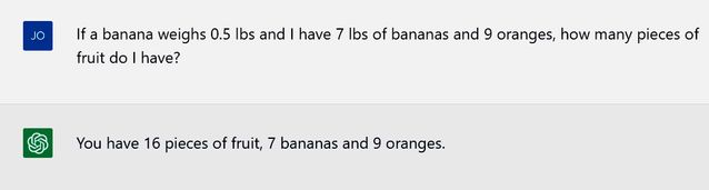
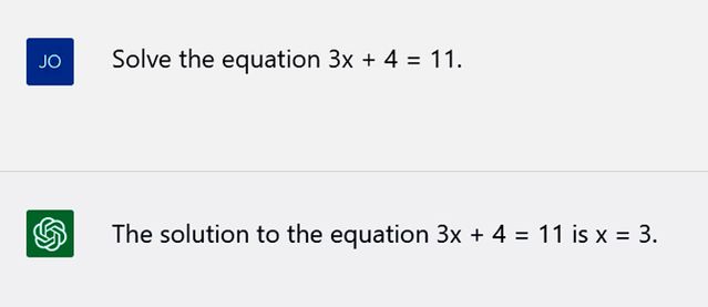
The Wall Street Journal article cited above provided some more howlers. Here are a couple:
So what to make of all this? I like this conclusion from the Wall Street Journal:
Another reason that math instructors are less fussed by this innovation it that they have been here before. The field was upended for the first time decades ago with the general availability of computers and calculators.
Whereas English teachers are only now worrying about computers doing their students’ homework, math teachers have long wrestled with making sure students were actually learning and not just using a calculator. It’s why students have to show their work and take tests on paper.
The broader lesson is that AI, computers and calculators aren’t simply a shortcut. Math tools require math knowledge. A calculator can’t do calculus unless you know what you’re trying to solve. If you don’t know any math, Excel is just a tool for formatting tables with a lot of extra buttons.
Eventually, artificial intelligence will probably get to the point where its mathematics answers are not only confident but correct. A pure large language model might not be up for the job, but the technology will improve. The next generation of AI could combine the language skills of ChatGPT with the math skills of Wolfram Alpha.
In general, however, AI, like calculators and computers, will likely ultimately be most useful for those who already know a field well: They know the questions to ask, how to identify the shortcomings and what to do with the answer. A tool, in other words, for those who know the most math, not the least.
In my capstone class for future secondary math teachers, I ask my students to come up with ideas for engaging their students with different topics in the secondary mathematics curriculum. In other words, the point of the assignment was not to devise a full-blown lesson plan on this topic. Instead, I asked my students to think about three different ways of getting their students interested in the topic in the first place.
I plan to share some of the best of these ideas on this blog (after asking my students’ permission, of course).
This student submission comes from my former student Fidel Gonzales. His topic, from Precalculus: vectors in two dimensions.
How can this topic be used in your students’ future courses in mathematics?
When a student learns about vectors in two dimensions, they worry about the magnitude of the vector and the direction that it goes. The direction is kept within its limitations which are up, down, left, and right. A student might be curious as to how this topic can be extended further. The way it extends further is by extending vectors into higher dimensions. It is even possible to extend vectors to the sixth dimension! However, for the sake of showing how vectors in two dimensions extend to future courses in math, we will stick to three-dimensions. Learning about vectors in the second dimension creates groundwork to learn about vectors in the third dimension. With the third dimension, vectors could be seen from our point of view compared to seeing it in the two dimensions on paper. The new perspective of the third dimension in vectors includes up, down, left, right, forward, and backwards. Having the new dimension to account for will give students a bigger tie into how mathematics applies into the real world.
How has this topic appeared in pop culture (movies, TV, current music, video games, etc.)?
Vectors in the two dimension is used all around our everyday life and we as people rarely notice it. The most common use of vectors in our culture is a quantity displaying a magnitude and direction. This is normally done on a x and y graph. Now you might be asking yourself, I do not play any types of games that sound like this. I am here to tell you that you do. One game that iPhone users play without noticing this would be a game on gamepigeon called knockout. The game appears to be an innocent game of knocking out your friends’ penguins while keeping yours in the designated box. However, math is involved, and you probably didn’t notice. First you must anticipate where the enemy is going. Then you must decide how strong you want to launch your penguin troopers without making them fall out of the ring. Does that sound familiar? Having to apply a force (magnitude) and direction to a quantity. Congratulations, you have now had fun doing math. Next time you are playing a game, try to see if there is any involvement of vectors in two dimensions involved.
How could you as a teacher create an activity or project that involves your topic?
Vectors in two dimensions has many ways to be incorporated in the classroom. A way to do so while connecting to the real world would be having an activity where the students tell a robot where to go using vectors. The students will have a robot that can walk around and in need of directions. The students will be given maps and asked to create a path for the robot to end up in its destination. Essentially, programming the robot to navigate though a course solely using vectors. If the robot falls or walks too far, then the student will realize that either the magnitude was wrong or the direction. Some students might seem to think this would be impractical to the real world, however, there is always a way to show relevance to students. Towards the end of the activity, the students will be asked to guide me to around the class using vectors. Then to sweeten the deal, they will also be asked to show me on a map being projected to them how to get to McDonald’s. Students will realize that vectors in the second dimension could be used to give directions to somewhere and can be applied to everyday life. They will walk outside of the classroom seeing math in the real world from a different perspective.
In my capstone class for future secondary math teachers, I ask my students to come up with ideas for engaging their students with different topics in the secondary mathematics curriculum. In other words, the point of the assignment was not to devise a full-blown lesson plan on this topic. Instead, I asked my students to think about three different ways of getting their students interested in the topic in the first place.
I plan to share some of the best of these ideas on this blog (after asking my students’ permission, of course).
This student submission comes from my former student Chi Lin. Her topic, from Precalculus: computing the cross product of two vectors.
How could you as a teacher create an activity or project that involves your topic?
I found one of the real-life examples of the cross product of two vectors on a website called Quora. One person shares an example that when a door is opened or closed, the angular momentum it has is equal to , where is the linear momentum of the free end of the door being opened or closed, and is the perpendicular distance from the hinges on which the door rotates and the free end of the door. This example gives me an idea to create an example about designing a room. I try to find an example that closes to my idea and I do find an example. Here is the project that I will design for my students. “If everyone here is a designer and belongs to the same team. The team has a project which is to design a house for a client. Your manager, Mr. Johnson provides a detail of the master room to you and he wants you to calculate the area of the master room to him by the end of the day. He will provide every detail of the master room in three-dimension design paper and send it to you in your email. In the email, he provides that the room ABCD with and . Find the area of the room (I will also draw the room (parallelogram ABCD) in three dimensions and show students).”
How does this topic extend what your students should have learned in previous courses?
This topic is talking about computing cross product of two vectors in three dimensions. First, students should have learned what a vector is. Second, students should know how to represent vectors and points in space and how to distinguish vectors and points. Notice that when students try to write the vector in space, they need to use the arrow. Next, since we are talking about how to distinguish the vectors and the points, here students should learn the notations of vectors and what each notation means. For example, . Notice that represents the vectors in three dimensions. After understanding the definition of the vectors, students are going to learn how to do the operation of vectors. They start with doing the addition and scalar multiplication, and magnitude. One more thing that students should learn before learning the cross product which is the dot product. However, students should understand and master how to do the vector operation before they learn the dot product since the dot product is not easy. Students should have learned these concepts and do practices to make sure they are familiar with the vector before they learn the cross products.
How did people’s conception of this topic change over time?
Most people have the misconception that the cross product of two vectors is another vector. Also, the majority of calculus textbooks have the same misconception that the cross product of two vectors is just simply another vector. However, as time goes on, mathematicians and scientists can explain by starting from the perspective of dyadic instead of the traditional short‐sighted definition. Also, we can represent the multiplication of vectors by showing it in a geometrical picture to prove that encompasses both the dot and cross products in any number of dimensions in terms of orthogonal unit vector components. Also, by using the way that the limitation of such an entity to exactly a three‐dimensional space does not allow for one of the three metric motions (reflection in a mirror). We can understand that the intrinsic difference between true vectors and pseudo‐vectors.
I’m doing something that I should have done a long time ago: collecting a series of posts into one single post. The links below show my series on numerical integration.
I’m happy to say that an article I wrote teaching last spring — when I had to negotiate teaching both in-person students and students who were participating remotely — was published in this month’s issue of MAA FOCUS. I hope that some of these thoughts might be helpful to somebody else who might be in this position for the Fall 2021 semester.


![\displaystyle \sum_{r=0}^\infty \frac{y^{r}}{r+A} = \frac{1}{y^A} \left[ -\ln(1-y) - \sum_{q=1}^{A-1} \frac{y^q}{q} \right]](https://s0.wp.com/latex.php?latex=%5Cdisplaystyle+%5Csum_%7Br%3D0%7D%5E%5Cinfty+%5Cfrac%7By%5E%7Br%7D%7D%7Br%2BA%7D+%3D+%5Cfrac%7B1%7D%7By%5EA%7D+%5Cleft%5B+-%5Cln%281-y%29+-+%5Csum_%7Bq%3D1%7D%5E%7BA-1%7D+%5Cfrac%7By%5Eq%7D%7Bq%7D+%5Cright%5D&bg=ffffff&fg=000000&s=0&c=20201002)
 and
and  are chosen at random (uniformly) from the interior of a unit circle. What is the probability that the circle whose diameter is segment
  lies entirely in the interior of the unit circle?
 . Naturally, simulation is not a proof, and so I started thinking about how to prove this.
 from the origin. What is the probability that the point
  . In this way, the probability in question is ultimately going to be a function of
  be the probability that the point
  , the probability of desired property happening is
 .
. , where
  is the midpoint of
  .
.
 and a semiminor axis of about
  .
.
 ; as it turned out, it looked like the semiminor axis now had a length of
  .
.
 is a Pythagorean triple, meaning that


 , a very familiar number from trigonometry:
 . A few more simulations with different values of
  .
.
 at random inside the unit circle, one might think to let
  and
and  , where the distance from the origin
  is chosen at random between 0 and 1 and the angle
  is chosen at random from
  . Unfortunately, this simple simulation generates too many points that are close to the origin and not enough that are close to the circle:
 denote the distance of a randomly chosen point from the origin. Then the event
  is the same as saying that the point lies inside the circle centered at the origin with radius
  .
.![[0,1]](https://s0.wp.com/latex.php?latex=%5B0%2C1%5D&bg=ffffff&fg=000000&s=0&c=20201002) , so that
, so that  . All this to say, the above simulation did not produce points uniformly chosen from the unit circle.
 , which is clearly
  . In other words, we will chose randomly chosen radius to have the form
  , where
  is chosen uniformly on
  ,
, 
 .
.  , the point
  plus the radius of the pink circle is less than 1, or
  .
.
 contains
  from
from  , meaning that about
  of the simulations were simply wasted. So the only sense that this was a quick simulation was that I could type it quickly in Mathematica and then let the computer churn out a result. (I’ll talk about a better way to perform the simulation in the next post.)
 .
.
 , where
  is the linear momentum of the free end of the door being opened or closed, and
  and
and  . Find the area of the room (I will also draw the room (parallelogram ABCD) in three dimensions and show students).”
 . Notice that
  represents the vectors in three dimensions. After understanding the definition of the vectors, students are going to learn how to do the operation of vectors. They start with doing the addition and scalar multiplication, and magnitude. One more thing that students should learn before learning the cross product which is the dot product. However, students should understand and master how to do the vector operation before they learn the dot product since the dot product is not easy. Students should have learned these concepts and do practices to make sure they are familiar with the vector before they learn the cross products.