Square roots and logarithms without a calculator (Part 12)

I recently came across the following computational trick: to estimate $\sqrt{b}$ , use

$\sqrt{b} \approx \displaystyle \frac{b+a}{2\sqrt{a}}$ ,

where $a$ is the closest perfect square to $b$ . For example,

$\sqrt{26} \approx \displaystyle \frac{26+25}{2\sqrt{25}} = 5.1$ .

I had not seen this trick before — at least stated in these terms — and I’m definitely not a fan of computational tricks without an explanation. In this case, the approximation is a straightforward consequence of a technique we teach in calculus. If $f(x) = (1+x)^n$ , then $f'(x) = n (1+x)^{n-1}$ , so that $f'(0) = n$ . Since $f(0) = 1$ , the equation of the tangent line to $f(x)$ at $x = 0$ is

$L(x) = f(0) + f'(0) \cdot (x-0) = 1 + nx$ .

The key observation is that, for $x \approx 0$ , the graph of $L(x)$ will be very close indeed to the graph of $f(x)$ . In Calculus I, this is sometimes called the linearization of $f$ at $x =a$ . In Calculus II, we observe that these are the first two terms in the Taylor series expansion of $f$ about $x = a$ .

For the problem at hand, if $n = 1/2$ , then

$\sqrt{1+x} \approx 1 + \displaystyle \frac{x}{2}$

if $x$ is close to zero. Therefore, if $a$ is a perfect square close to $b$ so that the relative difference $(b-a)/a$ is small, then

$\sqrt{b} = \sqrt{a + b - a}$

$= \sqrt{a} \sqrt{1 + \displaystyle \frac{b-a}{a}}$

$\approx \sqrt{a} \displaystyle \left(1 + \frac{b-a}{2a} \right)$

$= \sqrt{a} \displaystyle \left( \frac{2a + b-a}{2a} \right)$

$= \sqrt{a} \displaystyle \left( \frac{b+a}{2a} \right)$

$= \displaystyle \frac{b+a}{2\sqrt{a}}$ .

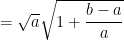
One more thought: All of the above might be a bit much to swallow for a talented but young student who has not yet learned calculus. So here’s another heuristic explanation that does not require calculus: if $a \approx b$ , then the geometric mean $\sqrt{ab}$ will be approximately equal to the arithmetic mean $(a+b)/2$ . That is,

$\sqrt{ab} \approx \displaystyle \frac{a+b}{2}$ ,

so that

$\sqrt{b} \approx \displaystyle \frac{a+b}{2\sqrt{a}}$ .

Square roots and logarithms without a calculator (Part 12)

Published by John Quintanilla

Leave a Reply Cancel reply

Share this:

Like this:

Related

Published by John Quintanilla

Leave a Reply Cancel reply