Numerical integration is a standard topic in first-semester calculus. From time to time, I have received questions from students on various aspects of this topic, including:
Why is numerical integration necessary in the first place?
Where do these formulas come from (especially Simpson’s Rule)?
How can I do all of these formulas quickly?
Is there a reason why the Midpoint Rule is better than the Trapezoid Rule?
Is there a reason why both the Midpoint Rule and the Trapezoid Rule converge quadratically?
Is there a reason why Simpson’s Rule converges like the fourth power of the number of subintervals?
In this series, I hope to answer these questions. While these are standard questions in a introductory college course in numerical analysis, and full and rigorous proofs can be found on Wikipedia and Mathworld, I will approach these questions from the point of view of a bright student who is currently enrolled in calculus and hasn’t yet taken real analysis or numerical analysis.
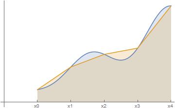
In this post, we will perform an error analysis for the Trapezoid Rule
where is the number of subintervals and is the width of each subinterval, so that .
As noted above, a true exploration of error analysis requires the generalized mean-value theorem, which perhaps a bit much for a talented high school student learning about this technique for the first time. That said, the ideas behind the proof are accessible to high school students, using only ideas from the secondary curriculum (especially the Binomial Theorem), if we restrict our attention to the special case , where is a positive integer.
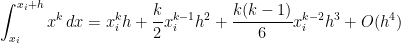
For this special case, the true area under the curve on the subinterval will be
In the above, the shorthand can be formally defined, but here we’ll just take it to mean “terms that have a factor of or higher that we’re too lazy to write out.” Since is supposed to be a small number, these terms will small in magnitude and thus can be safely ignored.
I wrote the above formula to include terms up to and including because I’ll need this later in this series of posts. For now, looking only at the Trapezoid Rule, it will suffice to write this integral as
.
Using the Trapezoid Rule, we approximate as , using the width and the bases and of the trapezoid. Using the Binomial Theorem, this expands as
Once again, this is a little bit overkill for the present purposes, but we’ll need this formula later in this series of posts. Truncating somewhat earlier, we find that the Trapezoid Rule for this subinterval gives
Subtracting from the actual integral, the error in this approximation will be equal to
In other words, like the Midpoint Rule, both of the first two terms and cancel perfectly, leaving us with a local error on the order of .
We also recall, from the previous post in this series that the local error from the Midpoint Rule was . In other words, while both the Midpoint Rule and Trapezoid Rule have local errors on the order of , we expect the error in the Midpoint Rule to be about half of the error from the Trapezoid Rule.
I'm a Professor of Mathematics and a University Distinguished Teaching Professor at the University of North Texas. For eight years, I was co-director of Teach North Texas, UNT's program for preparing secondary teachers of mathematics and science.
View all posts by John Quintanilla
Published
One thought on “Thoughts on Numerical Integration (Part 18): Trapezoid rule and local rate of convergence”

![\int_a^b f(x) \, dx \approx \frac{h}{2} \left[f(x_0) + 2f(x_1) + 2f(x_2) + \dots + 2f(x_{n-1}) +f(x_n) \right] \equiv T_n](https://s0.wp.com/latex.php?latex=%5Cint_a%5Eb+f%28x%29+%5C%2C+dx+%5Capprox+%5Cfrac%7Bh%7D%7B2%7D+%5Cleft%5Bf%28x_0%29+%2B+2f%28x_1%29+%2B+2f%28x_2%29+%2B+%5Cdots+%2B+2f%28x_%7Bn-1%7D%29+%2Bf%28x_n%29+%5Cright%5D+%5Cequiv+T_n&bg=ffffff&fg=000000&s=0&c=20201002)
 is the number of subintervals and
  is the width of each subinterval, so that
  .
.
 , where
  is a positive integer.
![[x_i, x_i +h]](https://s0.wp.com/latex.php?latex=%5Bx_i%2C+x_i+%2Bh%5D&bg=ffffff&fg=000000&s=0&c=20201002)
![\displaystyle \int_{x_i}^{x_i+h} x^k \, dx = \frac{1}{k+1} \left[ (x_i+h)^{k+1} - x_i^{k+1} \right]](https://s0.wp.com/latex.php?latex=%5Cdisplaystyle+%5Cint_%7Bx_i%7D%5E%7Bx_i%2Bh%7D+x%5Ek+%5C%2C+dx+%3D+%5Cfrac%7B1%7D%7Bk%2B1%7D+%5Cleft%5B+%28x_i%2Bh%29%5E%7Bk%2B1%7D+-+x_i%5E%7Bk%2B1%7D+%5Cright%5D&bg=ffffff&fg=000000&s=0&c=20201002)
![= \displaystyle \frac{1}{k+1} \left[x_i^{k+1} + {k+1 \choose 1} x_i^k h + {k+1 \choose 2} x_i^{k-1} h^2 + {k+1 \choose 3} x_i^{k-2} h^3 + {k+1 \choose 4} x_i^{k-3} h^4+ {k+1 \choose 5} x_i^{k-4} h^5+ O(h^6) - x_i^{k+1} \right]](https://s0.wp.com/latex.php?latex=%3D+%5Cdisplaystyle+%5Cfrac%7B1%7D%7Bk%2B1%7D+%5Cleft%5Bx_i%5E%7Bk%2B1%7D+%2B+%7Bk%2B1+%5Cchoose+1%7D+x_i%5Ek+h+%2B+%7Bk%2B1+%5Cchoose+2%7D+x_i%5E%7Bk-1%7D+h%5E2+%2B+%7Bk%2B1+%5Cchoose+3%7D+x_i%5E%7Bk-2%7D+h%5E3+%2B+%7Bk%2B1+%5Cchoose+4%7D+x_i%5E%7Bk-3%7D+h%5E4%2B+%7Bk%2B1+%5Cchoose+5%7D+x_i%5E%7Bk-4%7D+h%5E5%2B+O%28h%5E6%29+-+x_i%5E%7Bk%2B1%7D+%5Cright%5D&bg=ffffff&fg=000000&s=0&c=20201002)

![+ \displaystyle \frac{(k+1)k(k-1)(k-2)(k-3)}{120} x_i^{k-4} h^5 \bigg] + O(h^6)](https://s0.wp.com/latex.php?latex=%2B+%5Cdisplaystyle+%5Cfrac%7B%28k%2B1%29k%28k-1%29%28k-2%29%28k-3%29%7D%7B120%7D+x_i%5E%7Bk-4%7D+h%5E5+%5Cbigg%5D+%2B+O%28h%5E6%29+&bg=ffffff&fg=000000&s=0&c=20201002)

 can be formally defined, but here we’ll just take it to mean “terms that have a factor of
  or higher that we’re too lazy to write out.” Since
  is supposed to be a small number, these terms will small in magnitude and thus can be safely ignored.
I wrote the above formula to include terms up to and including
is supposed to be a small number, these terms will small in magnitude and thus can be safely ignored.
I wrote the above formula to include terms up to and including  because I’ll need this later in this series of posts. For now, looking only at the Trapezoid Rule, it will suffice to write this integral as
 as
as ![\displaystyle \frac{h}{2} \left[x_i^k + (x_i + h)^k \right]](https://s0.wp.com/latex.php?latex=%5Cdisplaystyle+%5Cfrac%7Bh%7D%7B2%7D+%5Cleft%5Bx_i%5Ek+%2B+%28x_i+%2B+h%29%5Ek+%5Cright%5D&bg=ffffff&fg=000000&s=0&c=20201002) , using the width
, using the width  and
and  of the trapezoid. Using the Binomial Theorem, this expands as


 and
and  cancel perfectly, leaving us with a local error on the order of
  .
We also recall, from the previous post in this series that the local error from the Midpoint Rule was
.
We also recall, from the previous post in this series that the local error from the Midpoint Rule was 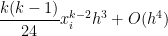 . In other words, while both the Midpoint Rule and Trapezoid Rule have local errors on the order of
  , we expect the error in the Midpoint Rule to be about half of the error from the Trapezoid Rule.

One thought on “Thoughts on Numerical Integration (Part 18): Trapezoid rule and local rate of convergence”