Thoughts on Numerical Integration (Part 2): The bell curve

Numerical integration is a standard topic in first-semester calculus. From time to time, I have received questions from students on various aspects of this topic, including:

Why is numerical integration necessary in the first place?
Where do these formulas come from (especially Simpson’s Rule)?
How can I do all of these formulas quickly?
Is there a reason why the Midpoint Rule is better than the Trapezoid Rule?
Is there a reason why both the Midpoint Rule and the Trapezoid Rule converge quadratically?
Is there a reason why Simpson’s Rule converges like the fourth power of the number of subintervals?

In this series, I hope to answer these questions. While these are standard questions in a introductory college course in numerical analysis, and full and rigorous proofs can be found on Wikipedia and Mathworld, I will approach these questions from the point of view of a bright student who is currently enrolled in calculus and hasn’t yet taken real analysis or numerical analysis.

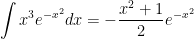
In this post, I’d like to take a closer look at the indefinite integral $\displaystyle \int e^{-x^2} dx$ , which is closely related to the area under the bell curve $\displaystyle \frac{1}{\sqrt{2\pi}} e^{-x^2/2} dx$ . This integral cannot be computed using elementary functions. However, using integration by parts, there are some related integrals that can be computed:

$\displaystyle \int x e^{-x^2} dx = -\displaystyle \frac{1}{2} e^{-x^2}$

$\displaystyle \int x^3 e^{-x^2} dx = -\displaystyle \frac{x^2+1}{2} e^{-x^2}$

$\displaystyle \int x^5 e^{-x^2} dx = -\displaystyle \frac{x^4+2x^2+2}{2} e^{-x^2}$

$\displaystyle \int x^7 e^{-x^2} dx = -\displaystyle \frac{x^6+3x^4+6x^2+6}{2} e^{-x^2}$

Based on these examples, it stands to reason that, if $\displaystyle \int e^{-x^2} dx$ can be written in terms of elementary functions, it should have the form

$\displaystyle \int e^{-x^2} dx = f(x) e^{-x^2}$ ,

where $f(x)$ is some polynomial to be determined. We will now show that this is impossible.

Suppose 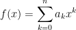$f(x) = \displaystyle \sum_{k=0}^n a_k x^k$ , a polynomial of degree $n$ to be determined. Then we have

$\displaystyle \frac{d}{dx} \left[ f(x) e^{-x^2} \right] = e^{-x^2}$

$f'(x) e^{-x^2} - 2 x f(x) e^{-x^2} =e^{-x^2}$

$f'(x) - 2x f(x) = 1$ .

In other words, all terms on the left-hand side except the constant term must cancel. However, this is impossible: $2x f(x)$ is a polynomial of degree $n+1$ while $f'(x)$ is a polynomial of degree $n-1$ . Therefore, the left hand side must have degree $n+1$ and therefore cannot be a constant.

A similar argument shows that 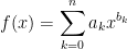$f(x)$ cannot have the form $f(x) = \displaystyle \sum_{k=0}^n a_k x^{b_k}$ , where the exponents $b_k$ may or may not be integers.

This may be enough to convince a calculus student that there is no elementary antiderivative of $\displaystyle e^{-x^2} dx$ . Indeed, although the proof goes well beyond first-year calculus, there is a theorem that says that if $\displaystyle \int x^a e^{bx^2}$ can be expressed in terms of elementary functions, then the antiderivative must have the form $f(x) e^{b x^2}$ . So the guess above actually can be rigorously justified. References:

Elena Anne Marchisotto and Gholam-Ali Zakeri, “An Invitation to Integration in Finite Terms,” The College Mathematics Journal , Sep., 1994, Vol. 25, No. 4 (Sep., 1994), pp. 295-308
J. F. Ritt, Integration in Finite Terms: Liouville’s Theory of Elementary Methods, Columbia University Press, New York, 1948

3 thoughts on “Thoughts on Numerical Integration (Part 2): The bell curve”

Thoughts on Numerical Integration (Part 2): The bell curve

Published by John Quintanilla

3 thoughts on “Thoughts on Numerical Integration (Part 2): The bell curve”

Leave a Reply Cancel reply

Share this:

Like this:

Related

Published by John Quintanilla

3 thoughts on “Thoughts on Numerical Integration (Part 2): The bell curve”

Leave a Reply Cancel reply