I’m in the middle of a series of posts concerning the elementary operation of computing a square root. In Part 3 of this series, I discussed how previous generations computed logarithms without a calculator by using log tables. In this post, I’ll discuss how previous generations computed, using the language of the time, antilogarithms. In Part 5, I’ll discuss my opinions about the pedagogical usefulness of log tables, even if logarithms can be computed more easily with scientific calculators. And in Part 6, I’ll return to square roots — specifically, how log tables can be used to find square roots.

Let’s again go back to a time before the advent of pocket calculators… say, 1943.

The following log tables come from one of my prized possessions: College Mathematics, by Kaj L. Nielsen (Barnes & Noble, New York, 1958).

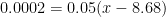
How to use the table, Part 5. The table can also be used to work backwards and find an antilogarithm. The term antilogarithm isn’t used much anymore, but the principle is still used in teaching students today. Suppose we wish to solve

, or .

Looking through the body of the table, we see that appears on the row marked and the column marked . Therefore, $10^{0.9509} \approx 8.93$. Again, this matches (to three and almost four significant digits) the result of a modern calculator.

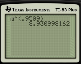
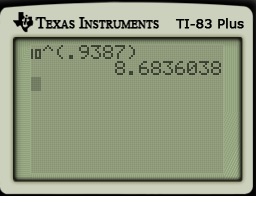
How to use the table, Part 6. Linear interpolation can also be used to find antilogarithms. Suppose we’re trying to evaluate ,  or find the value of so that $\log_{10} x = 0.9387$. From the table, we can trap between

and

So we again use linear interpolation, except this time the value of is known and the value of is unknown:

So we estimate This matches the result of a modern calculator to four significant digits:

How to use the table, Part 7.

How to use the table, Part 8.

Note: Sorry, but I’m not sure what happened… when the post came up this morning (August 4), I saw my work in Parts 7 and 8 had disappeared. Maybe one of these days I’ll restore this.