Thoughts on Numerical Integration (Part 19): Trapezoid rule and global rate of convergence

Numerical integration is a standard topic in first-semester calculus. From time to time, I have received questions from students on various aspects of this topic, including:

Why is numerical integration necessary in the first place?
Where do these formulas come from (especially Simpson’s Rule)?
How can I do all of these formulas quickly?
Is there a reason why the Midpoint Rule is better than the Trapezoid Rule?
Is there a reason why both the Midpoint Rule and the Trapezoid Rule converge quadratically?
Is there a reason why Simpson’s Rule converges like the fourth power of the number of subintervals?

In this series, I hope to answer these questions. While these are standard questions in a introductory college course in numerical analysis, and full and rigorous proofs can be found on Wikipedia and Mathworld, I will approach these questions from the point of view of a bright student who is currently enrolled in calculus and hasn’t yet taken real analysis or numerical analysis.

In the previous post, we showed that the Trapezoid Rule approximation of $\displaystyle \int_{x_i}^{x_i+h} x^k \, dx$ has error

$\displaystyle \frac{k(k-1)}{12} x_i^{k-2} h^3 + O(h^4)$

In this post, we consider the global error when integrating on the interval $[a,b]$ instead of a subinterval $[x_i,x_i+h]$ . The logic is almost a perfect copy-and-paste from the analysis used for the Midpoint Rule. The total error when approximating $\displaystyle \int_a^b x^k \, dx = \int_{x_0}^{x_n} x^k \, dx$ will be the sum of the errors for the integrals over $[x_0,x_1]$ , $[x_1,x_2]$ , through $[x_{n-1},x_n]$ . Therefore, the total error will be

$E \approx \displaystyle \frac{k(k-1)}{12} \left(x_0^{k-2} + x_1^{k-2} + \dots + x_{n-1}^{k-2} \right) h^3$ .

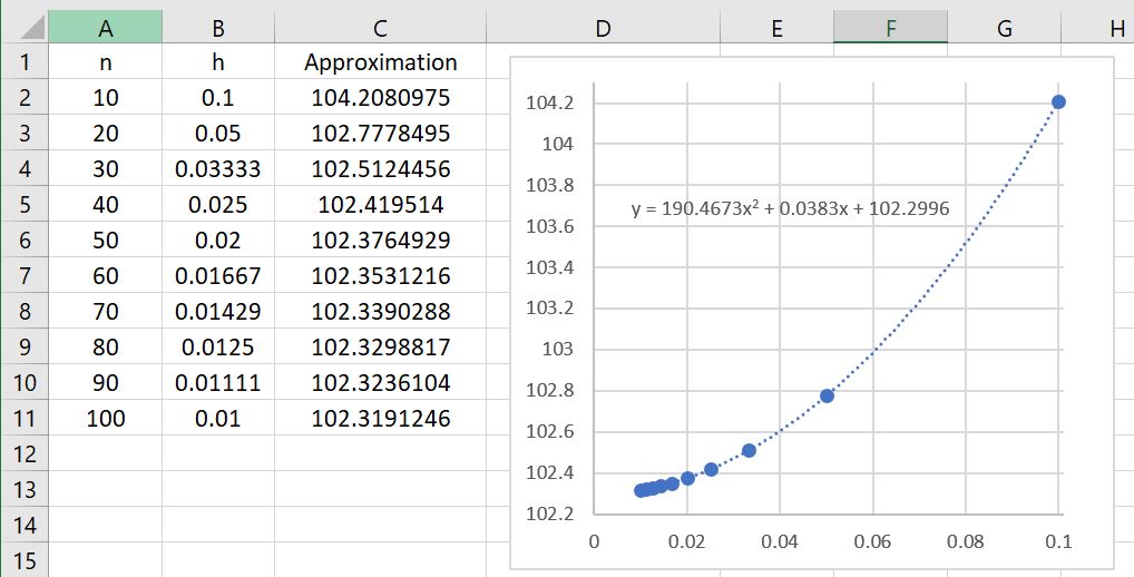
So that this formula doesn’t appear completely mystical, this actually matches the numerical observations that we made earlier. The figure below shows the left-endpoint approximations to $\displaystyle \int_1^2 x^9 \, dx$ for different numbers of subintervals. If we take $n = 100$ and $h = 0.01$ , then the error should be approximately equal to

$\displaystyle \frac{9 \times 8}{12} \left(1^7 + 1.01^7 + \dots + 1.99^7 \right) (0.01)^3 \approx 0.0187462$ ,

which, as expected, is close to the actual error of $102.3191246 - 102.3 \approx 0.0191246$ .

Let $y_i = x_i^{k-2}$ , so that the error becomes

$E \approx \displaystyle \frac{k(k-1)}{12} \left(y_0 + y_1 + \dots + y_{n-1} \right) h^3 + O(h^4) = \displaystyle \frac{k(k-1)}{12} \overline{y} n h^3$ ,

where $\overline{y} = (y_0 + y_1 + \dots + y_{n-1})/n$ is the average of the $y_i$ . Clearly, this average is somewhere between the smallest and the largest of the $y_i$ . Since $y = x^{k-2}$ is a continuous function, that means that there must be some value of $x_*$ between $x_0$ and $x_{k-1}$ — and therefore between $a$ and $b$ — so that $x_*^{k-2} = \overline{y}$ by the Intermediate Value Theorem. We conclude that the error can be written as

$E \approx \displaystyle \frac{k(k-1)}{12} x_*^{k-2} nh^3$ ,

Finally, since $h$ is the length of one subinterval, we see that $nh = b-a$ is the total length of the interval $[a,b]$ . Therefore,

$E \approx \displaystyle \frac{k(k-1)}{12} x_*^{k-2} (b-a)h^2 \equiv ch^2$ ,

where the constant $c$ is determined by $a$ , $b$ , and $k$ . In other words, for the special case $f(x) = x^k$ , we have established that the error from the Trapezoid Rule is approximately quadratic in $h$ — without resorting to the generalized mean-value theorem and confirming the numerical observations we made earlier.

One thought on “Thoughts on Numerical Integration (Part 19): Trapezoid rule and global rate of convergence”

Thoughts on Numerical Integration (Part 19): Trapezoid rule and global rate of convergence

Published by John Quintanilla

One thought on “Thoughts on Numerical Integration (Part 19): Trapezoid rule and global rate of convergence”

Leave a Reply Cancel reply

Share this:

Like this:

Related

Published by John Quintanilla

One thought on “Thoughts on Numerical Integration (Part 19): Trapezoid rule and global rate of convergence”

Leave a Reply Cancel reply