Numerical integration is a standard topic in first-semester calculus. From time to time, I have received questions from students on various aspects of this topic, including:
- Why is numerical integration necessary in the first place?
- Where do these formulas come from (especially Simpson’s Rule)?
- How can I do all of these formulas quickly?
- Is there a reason why the Midpoint Rule is better than the Trapezoid Rule?
- Is there a reason why both the Midpoint Rule and the Trapezoid Rule converge quadratically?
- Is there a reason why Simpson’s Rule converges like the fourth power of the number of subintervals?
In this series, I hope to answer these questions. While these are standard questions in a introductory college course in numerical analysis, and full and rigorous proofs can be found on Wikipedia and Mathworld, I will approach these questions from the point of view of a bright student who is currently enrolled in calculus and hasn’t yet taken real analysis or numerical analysis.

In the previous post in this series, I discussed three different ways of numerically approximating the definite integral 


In this series, we’ll choose equal-sized subintervals of the interval ![[a,b]](https://s0.wp.com/latex.php?latex=%5Ba%2Cb%5D&bg=ffffff&fg=000000&s=0&c=20201002)


![\int_a^b f(x) \, dx \approx h \left[f(x_0) + f(x_1) + \dots + f(x_{n-1}) \right] \equiv L_n](https://s0.wp.com/latex.php?latex=%5Cint_a%5Eb+f%28x%29+%5C%2C+dx+%5Capprox+h+%5Cleft%5Bf%28x_0%29+%2B+f%28x_1%29+%2B+%5Cdots+%2B+f%28x_%7Bn-1%7D%29+%5Cright%5D+%5Cequiv+L_n&bg=ffffff&fg=000000&s=0&c=20201002)
using left endpoints,
![\int_a^b f(x) \, dx \approx h \left[f(x_1) + f(x_2) + \dots + f(x_n) \right] \equiv R_n](https://s0.wp.com/latex.php?latex=%5Cint_a%5Eb+f%28x%29+%5C%2C+dx+%5Capprox+h+%5Cleft%5Bf%28x_1%29+%2B+f%28x_2%29+%2B+%5Cdots+%2B+f%28x_n%29+%5Cright%5D+%5Cequiv+R_n&bg=ffffff&fg=000000&s=0&c=20201002)
using right endpoints, and
![\int_a^b f(x) \, dx \approx h \left[f(c_1) + f(c_2) + \dots + f(c_n) \right] \equiv M_n](https://s0.wp.com/latex.php?latex=%5Cint_a%5Eb+f%28x%29+%5C%2C+dx+%5Capprox+h+%5Cleft%5Bf%28c_1%29+%2B+f%28c_2%29+%2B+%5Cdots+%2B+f%28c_n%29+%5Cright%5D+%5Cequiv+M_n&bg=ffffff&fg=000000&s=0&c=20201002)
using the midpoints of the subintervals. We have also derived the Trapezoid Rule
![\int_a^b f(x) \, dx \approx \displaystyle \frac{h}{2} [f(x_0) + 2f(x_1) + \dots + 2f(x_{n-1}) + f(x_n)] \equiv T_n](https://s0.wp.com/latex.php?latex=%5Cint_a%5Eb+f%28x%29+%5C%2C+dx+%5Capprox+%5Cdisplaystyle+%5Cfrac%7Bh%7D%7B2%7D+%5Bf%28x_0%29+%2B+2f%28x_1%29+%2B+%5Cdots+%2B+2f%28x_%7Bn-1%7D%29+%2B+f%28x_n%29%5D+%5Cequiv+T_n&bg=ffffff&fg=000000&s=0&c=20201002)
and Simpson’s Rule (if 
![\int_a^b f(x) \, dx \approx \displaystyle \frac{h}{3} \left[y_0 + 4 y_1 + 2 y_2 + 4 y_3 + \dots + 2y_{n-2} + 4 y_{n-1} + y_{n} \right] \equiv S_n](https://s0.wp.com/latex.php?latex=%5Cint_a%5Eb+f%28x%29+%5C%2C+dx+%5Capprox+%5Cdisplaystyle+%5Cfrac%7Bh%7D%7B3%7D+%5Cleft%5By_0+%2B+4+y_1+%2B+2+y_2+%2B+4+y_3+%2B+%5Cdots+%2B+2y_%7Bn-2%7D+%2B+4+y_%7Bn-1%7D+%2B%C2%A0+y_%7Bn%7D+%5Cright%5D+%5Cequiv+S_n&bg=ffffff&fg=000000&s=0&c=20201002)
![]() All of the above approximations to
All of the above approximations to 


 Unfortunately, simply taking more subintervals has its limitations. Using a spreadsheet as in the previous post in this series, one can implement 100 or even 1000 subintervals without much difficult. However, as demonstrated in the video below, implementing any of these methods with 10,000 subintervals is pretty time-consuming. (Tl/dw: It can take literally a couple of minutes.)
Instead of relying on sheer computational firepower, let’s instead investigate how good these numerical methods actually are. To begin, let’s explore the left-endpoint rule applied to 
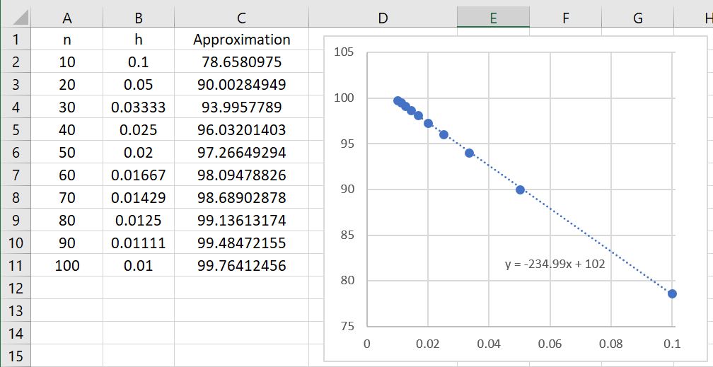 As
As 

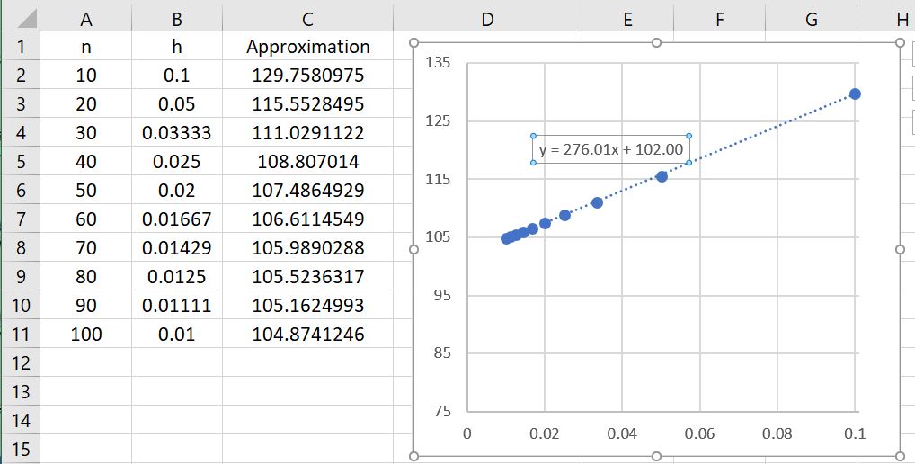 So, it appears that the errors in both the left- and right-endpoint rules are a linear function of the size of the subintervals. Said another way, if twice as many subintervals are taken, then the error appears to go down by a factor of 2. If ten times as many subintervals are used, then the error should go down by a factor of 10. As we’ll see in the next few posts, the errors for the Midpoint Rule, the Trapezoid Rule, and especially Simpson’s Rule are much better than the errors from these two methods.

One thought on “Thoughts on Numerical Integration (Part 8): Left and right endpoint rules and exploration of error analysis”