Thoughts on Numerical Integration (Part 15): Right endpoint rule and global rate of convergence

Numerical integration is a standard topic in first-semester calculus. From time to time, I have received questions from students on various aspects of this topic, including:

Why is numerical integration necessary in the first place?
Where do these formulas come from (especially Simpson’s Rule)?
How can I do all of these formulas quickly?
Is there a reason why the Midpoint Rule is better than the Trapezoid Rule?
Is there a reason why both the Midpoint Rule and the Trapezoid Rule converge quadratically?
Is there a reason why Simpson’s Rule converges like the fourth power of the number of subintervals?

In this series, I hope to answer these questions. While these are standard questions in a introductory college course in numerical analysis, and full and rigorous proofs can be found on Wikipedia and Mathworld, I will approach these questions from the point of view of a bright student who is currently enrolled in calculus and hasn’t yet taken real analysis or numerical analysis.

In the previous post in this series, we found that the local error of the right endpoint approximation to $\displaystyle \int_{x_i}^{x_i+h} x^k \, dx$ was equal to

$\displaystyle \frac{k}{2} x_i^{k-1} h^2 + O(h^3)$ .

The total error when approximating $\displaystyle \int_a^b x^k \, dx = \int_{x_0}^{x_n} x^k , dx$ will be the sum of the errors for the integrals over $[x_0,x_1]$ , $[x_1,x_2]$ , through $[x_{n-1},x_n]$ . Therefore, the total error will be

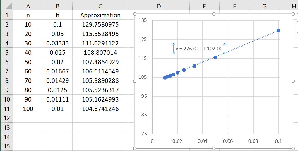
$E \approx \displaystyle \frac{k}{2} \left(x_1^{k-1} + x_2^{k-1} + \dots + x_{n}^{k-1} \right) h^2$ .

So that this formula doesn’t appear completely mystical, this actually matches the numerical observations that we made earlier. The figure below shows the left-endpoint approximations to $\displaystyle \int_1^2 x^9 \, dx$ for different numbers of subintervals. If we take $n = 100$ and $h = 0.01$ , then the error should be approximately equal to

$\displaystyle \frac{9}{2} \left(1.01^8 + 1.02^8 + \dots + 2^8 \right) (0.01)^2 \approx 2.61276$ ,

which, as expected, is close to the actual error of $104.8741246 - 102.3 \approx 2.57412$ .

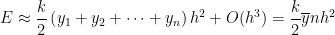
We now perform a more detailed analysis of the global error, which is almost a perfect copy-and-paste from the previous analysis. Let $y_i = x_i^{k-1}$ , so that the error becomes

$E \approx \displaystyle \frac{k}{2} \left(y_1 + y_2 + \dots + y_n \right) h^2 + O(h^3) = \displaystyle \frac{k}{2} \overline{y} n h^2$ ,

where $\overline{y} = (y_1 + y_2 + \dots + y_{n})/n$ is the average of the $y_i$ . Clearly, this average is somewhere between the smallest and the largest of the $y_i$ . Since $y = x^{k-1}$ is a continuous function, that means that there must be some value of $x_*$ between $x_1$ and $x_{n}$ — and therefore between $a$ and $b$ — so that $x_*^{k-1} = \overline{y}$ by the Intermediate Value Theorem. We conclude that the error can be written as

$E \approx \displaystyle \frac{k}{2} x_*^{k-1} nh^2$ ,

Finally, since $h$ is the length of one subinterval, we see that $nh = b-a$ is the total length of the interval $[a,b]$ . Therefore,

$E \approx \displaystyle \frac{k}{2} x_*^{k-1} (b-a)h \equiv ch$ ,

where the constant $c$ is determined by $a$ , $b$ , and $k$ . In other words, for the special case $f(x) = x^k$ , we have established that the error from the left-endpoint rule is approximately linear in $h$ — without resorting to the generalized mean-value theorem.

One thought on “Thoughts on Numerical Integration (Part 15): Right endpoint rule and global rate of convergence”

Thoughts on Numerical Integration (Part 15): Right endpoint rule and global rate of convergence

Published by John Quintanilla

One thought on “Thoughts on Numerical Integration (Part 15): Right endpoint rule and global rate of convergence”

Leave a Reply Cancel reply

Share this:

Like this:

Related

Published by John Quintanilla

One thought on “Thoughts on Numerical Integration (Part 15): Right endpoint rule and global rate of convergence”

Leave a Reply Cancel reply