Thoughts on Numerical Integration (Part 9): Midpoint rule and exploration of error analysis

Numerical integration is a standard topic in first-semester calculus. From time to time, I have received questions from students on various aspects of this topic, including:

• Why is numerical integration necessary in the first place?
• Where do these formulas come from (especially Simpson’s Rule)?
• How can I do all of these formulas quickly?
• Is there a reason why the Midpoint Rule is better than the Trapezoid Rule?
• Is there a reason why both the Midpoint Rule and the Trapezoid Rule converge quadratically?
• Is there a reason why Simpson’s Rule converges like the fourth power of the number of subintervals?

In this series, I hope to answer these questions. While these are standard questions in a introductory college course in numerical analysis, and full and rigorous proofs can be found on Wikipedia and Mathworld, I will approach these questions from the point of view of a bright student who is currently enrolled in calculus and hasn’t yet taken real analysis or numerical analysis.

In the previous post in this series, I discussed three different ways of numerically approximating the definite integral , the area under a curve between and .

In this series, we’ll choose equal-sized subintervals of the interval . If is the width of each subinterval so that , then the integral may be approximated as

using left endpoints,

using right endpoints, and

using the midpoints of the subintervals. We have also derived the Trapezoid Rule

and Simpson’s Rule (if is even)

.

In the previous post in this series, we saw that both the left-endpoint and right-endpoint rules have a linear rate of convergence: if twice as many subintervals are taken, then the error appears to go down by a factor of 2. If ten times as many subintervals are used, then the error should go down by a factor of 10. Let’s now explore the results of the midpoint rule applied to using different numbers of subintervals. The results are summarized in the table below. 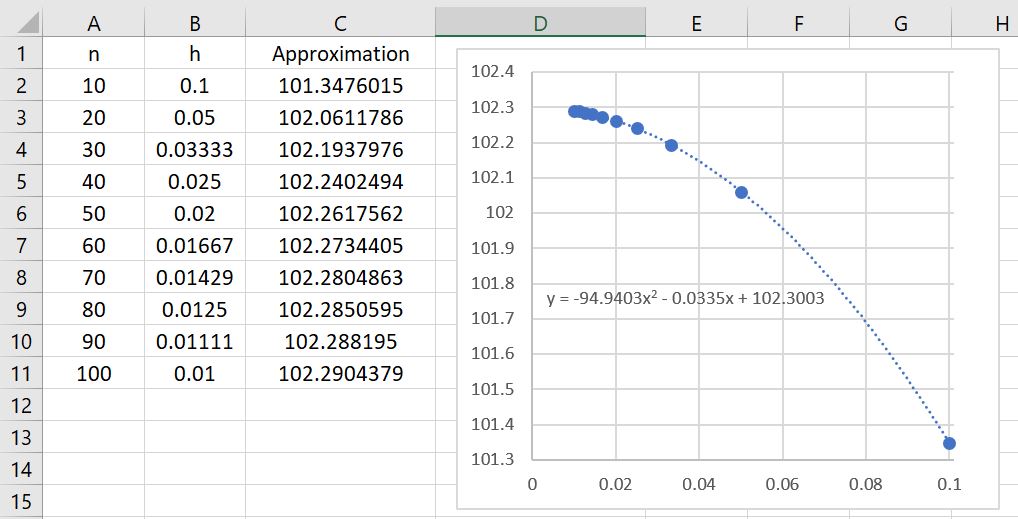The first immediate observation is that these approximations are far better than the left- and right-endpoint rule approximations! Indeed, we see that , using only ten subintervals, is a far better approximation than (from the previous post) either or using 100 subintervals! The lesson to learn: choosing a good algorithm is often far better than simply doing lots of computations.

There’s a second observation: the rate of convergence appears to be much, much faster. Indeed, the data points appear to fit a parabola very well instead of a straight line. Said another way, if twice as many subintervals are taken, then the error appears to go down by a factor of 4. If ten times as many subintervals are used, then the error should go down by a factor of 100. This illustrates quadratic convergence, as opposed to the mere linear convergence of the left- and right-endpoint rules.