Thoughts on Numerical Integration (Part 4): Derivation of Trapezoid Rule

Numerical integration is a standard topic in first-semester calculus. From time to time, I have received questions from students on various aspects of this topic, including:

Why is numerical integration necessary in the first place?
Where do these formulas come from (especially Simpson’s Rule)?
How can I do all of these formulas quickly?
Is there a reason why the Midpoint Rule is better than the Trapezoid Rule?
Is there a reason why both the Midpoint Rule and the Trapezoid Rule converge quadratically?
Is there a reason why Simpson’s Rule converges like the fourth power of the number of subintervals?

In this series, I hope to answer these questions. While these are standard questions in a introductory college course in numerical analysis, and full and rigorous proofs can be found on Wikipedia and Mathworld, I will approach these questions from the point of view of a bright student who is currently enrolled in calculus and hasn’t yet taken real analysis or numerical analysis.

In the previous post in this series, I discussed three different ways of numerically approximating the definite integral $\displaystyle \int_a^b f(x) \, dx$ , the area under a curve $f(x)$ between $x=a$ and $x=b$ .

In this series, we’ll choose equal-sized subintervals of the interval $[a,b]$ . If $h = (b-a)/n$ is the width of each subinterval so that $x_k = x_0 + kh$ , then the integral may be approximated as

$\int_a^b f(x) \, dx \approx h \left[f(x_0) + f(x_1) + \dots + f(x_{n-1}) \right] \equiv L_n$

using left endpoints,

$\int_a^b f(x) \, dx \approx h \left[f(x_1) + f(x_2) + \dots + f(x_n) \right] \equiv R_n$

using right endpoints, and

$\int_a^b f(x) \, dx \approx h \left[f(c_1) + f(c_2) + \dots + f(c_n) \right] \equiv M_n$

using the midpoints of the subintervals.

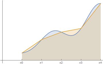
All three of these approximations were obtained by approximating the above shaded region by rectangles. However, perhaps it might be better to use some other shape besides rectangles. In the Trapezoidal Rule, we approximate the area by using (surprise!) trapezoids, as in the figure below.

The first trapezoid has height $h$ and bases $f(x_0)$ and $f(x_1)$ , and so the area of the first trapezoid is $\frac{1}{2} h[ f(x_0) + f(x_1) ]$ . The other areas are found similarly. Adding these together, we get the approximation

$T_n = \displaystyle \frac{h}{2}[f(x_0) + f(x_1)] + \frac{h}{2} [f(x_1) + f(x_2)] + \dots +$

$+ \displaystyle \frac{h}{2} [f(x_{n-2})+f(x_{n-1})] + \frac{h}{2} [f(x_{n-1})+f(x_n)]$

$= \displaystyle \frac{h}{2} [f(x_0) + 2f(x_1) + 2f(x_2) + \dots + 2f(x_{n-2}) + 2f(x_{n-1}) + f(x_n)].$

Interestingly, $T_n$ is the average of the two endpoint approximations $L_n$ and $R_n$ :

$\displaystyle \frac{L_n+R_n}{2} = \frac{L_n}{2} + \frac{R_n}{2}$

$= \displaystyle \frac{h}{2} \left[f(x_0) + f(x_1) + f(x_2) + \dots + f(x_{n-1}) \right]$

$+\displaystyle \frac{h}{2} \left[f(x_1) + f(x_2) + \dots + f(x_{n-1}) + f(x_{n}) \right]$

$= \displaystyle \frac{h}{2} \left[f(x_0) + 2f(x_1) + \dots + 2f(x_{n-1}) + f(x_n) \right]$

$= T_n$ .

Of course, as a matter of computation, it’s a lot quicker to directly compute $T_n$ instead of computing $L_n$ and $R_n$ separately and then averaging.

One thought on “Thoughts on Numerical Integration (Part 4): Derivation of Trapezoid Rule”

Thoughts on Numerical Integration (Part 4): Derivation of Trapezoid Rule

Published by John Quintanilla

One thought on “Thoughts on Numerical Integration (Part 4): Derivation of Trapezoid Rule”

Leave a Reply Cancel reply

Share this:

Like this:

Related

Published by John Quintanilla

One thought on “Thoughts on Numerical Integration (Part 4): Derivation of Trapezoid Rule”

Leave a Reply Cancel reply