Thoughts on Numerical Integration (Part 11): Simpson’s Rule and exploration of error analysis

Numerical integration is a standard topic in first-semester calculus. From time to time, I have received questions from students on various aspects of this topic, including:

• Why is numerical integration necessary in the first place?
• Where do these formulas come from (especially Simpson’s Rule)?
• How can I do all of these formulas quickly?
• Is there a reason why the Midpoint Rule is better than the Trapezoid Rule?
• Is there a reason why both the Midpoint Rule and the Trapezoid Rule converge quadratically?
• Is there a reason why Simpson’s Rule converges like the fourth power of the number of subintervals?

In this series, I hope to answer these questions. While these are standard questions in a introductory college course in numerical analysis, and full and rigorous proofs can be found on Wikipedia and Mathworld, I will approach these questions from the point of view of a bright student who is currently enrolled in calculus and hasn’t yet taken real analysis or numerical analysis.

In the previous post in this series, I discussed three different ways of numerically approximating the definite integral , the area under a curve between and .

In this series, we’ll choose equal-sized subintervals of the interval . If is the width of each subinterval so that , then the integral may be approximated as

using left endpoints,

using right endpoints, and

using the midpoints of the subintervals. We have also derived the Trapezoid Rule

and Simpson’s Rule (if is even)

.

In the previous post in this series, we saw that both the left-endpoint and right-endpoint rules have a linear rate of convergence: if twice as many subintervals are taken, then the error appears to go down by a factor of 2. If ten times as many subintervals are used, then the error should go down by a factor of 10. However, both the Midpoint Rule and the Trapezoid Rule have a quadratic rate of convergence: if twice as many subintervals are taken, then the error appears to go down by a factor of 4. If ten times as many subintervals are used, then the error should go down by a factor of 100. Moreover, it appears that the error from the Midpoint Rule is about half that of the Trapezoid Rule if the same number of subintervals are used.

Let’s now explore the results of Simpson’s Rule applied to using different numbers of subintervals. The results are summarized in the table below.

 

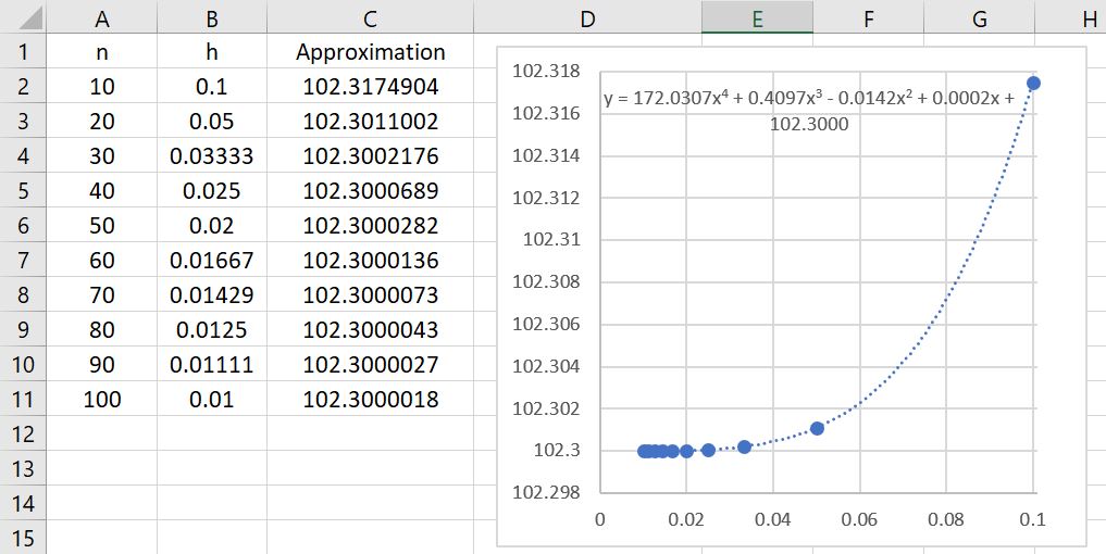
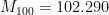
The first immediate observation is that these approximations are far better than even the Midpoint and Trapezoid Rules! Indeed, we see that , using only 20 subintervals, is a better approximation than (from previous posts) either or using 100 subintervals! The lesson to learn again: Simpson’s Rule is a bit more difficult to compute than the Trapezoid Rule or the Midpoint Rule because of the different weights. Nevertheless, choosing a good algorithm is often far better than simply doing lots of computations.

There’s a second observation: the rate of convergence appears to be much, much faster. Indeed, the data points appear to fit a quartic polynomial very well. Said another way, if twice as many subintervals are taken, then the error appears to go down by a factor of 16. We can actually see this in the figure, looking at the lines with 10, 20, 40, and 80 subintervals.

Error with 10 subintervals = .

Error with 20 subintervals = .

Error with 40 subintervals = .

Error with 80 subintervals = .

In all cases, the error on the next line is about the error on the previous line divided by 16.

This illustrates quartic convergence, as opposed to the mere linear convergence of the left- and right-endpoint rules or the quadratic convergence of the Midpoint and Trapezoid Rules.