Numerical integration is a standard topic in first-semester calculus. From time to time, I have received questions from students on various aspects of this topic, including:
- Why is numerical integration necessary in the first place?
- Where do these formulas come from (especially Simpson’s Rule)?
- How can I do all of these formulas quickly?
- Is there a reason why the Midpoint Rule is better than the Trapezoid Rule?
- Is there a reason why both the Midpoint Rule and the Trapezoid Rule converge quadratically?
- Is there a reason why Simpson’s Rule converges like the fourth power of the number of subintervals?
In this series, I hope to answer these questions. While these are standard questions in a introductory college course in numerical analysis, and full and rigorous proofs can be found on Wikipedia and Mathworld, I will approach these questions from the point of view of a bright student who is currently enrolled in calculus and hasn’t yet taken real analysis or numerical analysis.

In this series, we have shown the following approximations of errors when using various numerical approximations for 
As we now present, the formulas that we derived are (of course) easily connected to known theorems for the convergence of these techniques. These proofs, however, require some fairly advanced techniques from calculus. So, while the formulas derived in this series of posts only apply to 
Left and right endpoints: Our formula was
 ,
,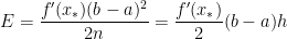 .
. .
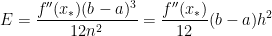
.![]() Midpoint Rule: Our formula was
Midpoint Rule: Our formula was

where 


This reduces to the formula that we derived since 
Trapezoid Rule: Our formula was

where
This reduces to the formula that we derived since
This reduces to the formula that we derived since
Simpson’s Rule: Our formula was
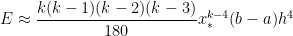
where
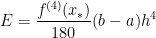
This reduces to the formula that we derived since 

One thought on “Thoughts on Numerical Integration (Part 22): Comparison to theorems about magnitudes of errors”