Thoughts on Numerical Integration (Part 20): Simpson’s rule and local rate of convergence

Numerical integration is a standard topic in first-semester calculus. From time to time, I have received questions from students on various aspects of this topic, including:

Why is numerical integration necessary in the first place?
Where do these formulas come from (especially Simpson’s Rule)?
How can I do all of these formulas quickly?
Is there a reason why the Midpoint Rule is better than the Trapezoid Rule?
Is there a reason why both the Midpoint Rule and the Trapezoid Rule converge quadratically?
Is there a reason why Simpson’s Rule converges like the fourth power of the number of subintervals?

In this series, I hope to answer these questions. While these are standard questions in a introductory college course in numerical analysis, and full and rigorous proofs can be found on Wikipedia and Mathworld, I will approach these questions from the point of view of a bright student who is currently enrolled in calculus and hasn’t yet taken real analysis or numerical analysis.

In this post, we will perform an error analysis for Simpson’s Rule

$\int_a^b f(x) \, dx \approx \frac{h}{3} \left[f(x_0) + 4(x_1) + 2f(x_2) + \dots + 2f(x_{n-2}) + 4f(x_{n-1}) +f(x_n) \right] \equiv T_n$

where $n$ is the number of subintervals (which has to be even) and $h = (b-a)/n$ is the width of each subinterval, so that $x_k = x_0 + kh$ .

For this special case, the true area under the curve $f(x) = x^k$ on the subinterval $[x_i, x_i +h]$ will be

$\displaystyle \int_{x_i}^{x_i+h} x^k \, dx = \frac{1}{k+1} \left[ (x_i+h)^{k+1} - x_i^{k+1} \right]$

$= \displaystyle \frac{1}{k+1} \left[x_i^{k+1} + {k+1 \choose 1} x_i^k h + {k+1 \choose 2} x_i^{k-1} h^2 + {k+1 \choose 3} x_i^{k-2} h^3 + {k+1 \choose 4} x_i^{k-3} h^4+ {k+1 \choose 5} x_i^{k-4} h^5+ O(h^6) - x_i^{k+1} \right]$

$= \displaystyle \frac{1}{k+1} \bigg[ (k+1) x_i^k h + \frac{(k+1)k}{2} x_i^{k-1} h^2 + \frac{(k+1)k(k-1)}{6} x_i^{k-2} h^3+ \frac{(k+1)k(k-1)(k-2)}{24} x_i^{k-3} h^4$

$+ \displaystyle \frac{(k+1)k(k-1)(k-2)(k-3)}{120} x_i^{k-4} h^5 \bigg] + O(h^6)$

$= x_i^k h + \displaystyle \frac{k}{2} x_i^{k-1} h^2 + \frac{k(k-1)}{6} x_i^{k-2} h^3 + \frac{k(k-1)(k-2)}{24} x_i^{k-3} h^4 + \frac{k(k-1)(k-2)(k-3)}{120} x_i^{k-4} h^5 + O(h^6)$

In the above, the shorthand $O(h^6)$ can be formally defined, but here we’ll just take it to mean “terms that have a factor of $h^6$ or higher that we’re too lazy to write out.” Since $h$ is supposed to be a small number, these terms will small in magnitude and thus can be safely ignored.

Earlier in this series, we derived the very convenient relationship $S_{2n} = \displaystyle \frac{2}{3} M_n + \frac{1}{3} T_n$ relating the approximations from Simpson’s Rule, the Midpoint Rule, and the Trapezoid Rule. We now exploit this relationship to approximate $\displaystyle \int_{x_i}^{x_i+h} x^k \, dx$ . Earlier in this series, we found the Midpoint Rule approximation on this subinterval to be

$M = x_i^k h + \displaystyle \frac{k}{2} x_i^{k-1} h^2 + \frac{k(k-1)}{8} x_i^{k-2} h^3 + \frac{k(k-1)(k-2}{48} x_i^{k-3} h^4$

$\displaystyle + \frac{k(k-1)(k-2)(k-3)}{384} x_i^{k-4} h^5 + O(h^6)$

while we found the Trapezoid Rule approximation to be

$T = x_i^k h + \displaystyle \frac{k}{2} x_i^{k-1} h^2 + \frac{k(k-1)}{4} x_i^{k-2} h^3 + \frac{k(k-1)(k-2)}{12} x_i^{k-3} h^4$

$\displaystyle + \frac{k(k-1)(k-2)(k-3)}{48} x_i^{k-4} h^5 + O(h^6)$ .

Therefore, if there are $2n$ subintervals, the Simpson’s Rule approximation of $\displaystyle \int_{x_i}^{x_i+h} x^k \, dx$ — that is, the area under the parabola that passes through $(x_i, x_i^k)$ , $(x_i + h/2, (x_i +h/2)^k)$ , and $(x_i + h, (x_i +h)^k)$ — will be $S = \frac{2}{3}M + \frac{1}{3}T$ . Since

$\displaystyle \frac{2}{3} \frac{1}{8} + \frac{1}{3} \frac{1}{4} = \frac{1}{6}$ ,

$\displaystyle \frac{2}{3} \frac{1}{48} + \frac{1}{3} \frac{1}{12} = \frac{1}{24}$ ,

and

$\displaystyle \frac{2}{3} \frac{1}{384} + \frac{1}{3} \frac{1}{48} = \frac{5}{576}$ ,

we see that

$S = x_i^k h + \displaystyle \frac{k}{2} x_i^{k-1} h^2 + \frac{k(k-1)}{6} x_i^{k-2} h^3 + \frac{k(k-1)(k-2)}{24} x_i^{k-3} h^4$

$\displaystyle + \frac{5k(k-1)(k-2)(k-3)}{576} x_i^{k-4} h^5 + O(h^6)$ .

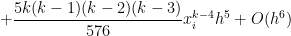
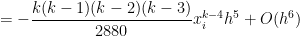
We notice that something wonderful just happened: the first four terms of $S$ perfectly match the first four terms of the exact value of the integral! Subtracting from the actual integral, the error in this approximation will be equal to

$\displaystyle \frac{k(k-1)(k-2)(k-3)}{120} x_i^{k-4} h^5 - \frac{5k(k-1)(k-2)(k-3)}{576} x_i^{k-4} h^5 + O(h^6)$

$= -\displaystyle \frac{k(k-1)(k-2)(k-3)}{2880} x_i^{k-4} h^5 + O(h^6)$

Before moving on, there’s one minor bookkeeping issue to deal with. We note that this is the error for $S_{2n}$ , where $2n$ subintervals are used. However, the value of $h$ in this equal arose from $T_n$ and $M_n$ , where only $n$ subintervals are used. So let’s write the error with $2n$ subintervals as

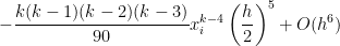
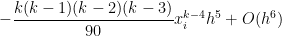
$-\displaystyle \frac{k(k-1)(k-2)(k-3)}{90} x_i^{k-4} \left( \frac{h}{2} \right)^5 + O(h^6)$ ,

where $h/2$ is the width of all of the $2n$ subintervals. By analogy, we see that the error for $n$ subintervals will be

$-\displaystyle \frac{k(k-1)(k-2)(k-3)}{90} x_i^{k-4} h^5 + O(h^6)$ .

But even after adjusting for this constant, we see that this local error behaves like $O(h^5)$ , a vast improvement over both the Midpoint Rule and the Trapezoid Rule. This illustrates a general principle of numerical analysis: given two algorithms that are $O(h^3)$ , an improved algorithm can typically be made by taking some linear combination of the two algorithms. Usually, the improvement will be to $O(h^4)$ ; however, in this example, we magically obtained an improvement to $O(h^5)$ .

One thought on “Thoughts on Numerical Integration (Part 20): Simpson’s rule and local rate of convergence”

Pingback: Thoughts on Numerical Integration: Index – Mean Green Math

Thoughts on Numerical Integration (Part 20): Simpson’s rule and local rate of convergence

Published by John Quintanilla

One thought on “Thoughts on Numerical Integration (Part 20): Simpson’s rule and local rate of convergence”

Leave a Reply Cancel reply

Share this:

Like this:

Related

Published by John Quintanilla

One thought on “Thoughts on Numerical Integration (Part 20): Simpson’s rule and local rate of convergence”

Leave a Reply Cancel reply