After finishing the Product, Quotient, and Chain Rules in my calculus class, I’d tell my class the following: “Next time, we’re going to play Stump the Prof. Anything that you can write on the board in 15 seconds, I will differentiate. Anything. I don’t care how hard it looks, I’ll differentiate it (if it has a derivative). So do your best to stump me.”
At the next lecture, I would devote the last 15-20 minutes of class time to Stump the Prof. Students absolutely loved it… their competitive juices got flowing as they tried to think of the nastiest, hairiest functions that they could write on the board in 15 seconds. And I’d differentiate them all using the rules we’d just covered.. though I never promised that I would simplify the derivatives!
Sometimes the results were quite funny. Every once in a while, a student would write some amazingly awful expression but forgot to include an 
The worst one I ever got was something like this:

Differentiating this took a good 3-4 minutes and took maybe 5 lines across the entire length of the chalkboard; I remember that my arm was sore after writing down the derivative. Naturally, some wise guy used his 15 seconds to write 
The point of this exercise is to illustrate to students that differentiation is a science; there are rules to follow, and by carefully following the rules, one can find the derivative of any “standard” function.
Later on, when we hit integration, I’ll draw a contrast: differentiation is a science, but integration is a combination of both science and art.


 , and the substitution
  .
. .
. , the magic substitution
  :
:
 .
. and diverges for
  . The boundary of
  , on the other hand, has to be checked separately for convergence.
 into the geometric series
 ,
, .
.

 and not to
  . Here’s the sum up to 10,000 terms… the entry in column E is the first few digits in the decimal expansion of
  .
. 
 , and there’s good visual evidence to think that the answer is
  is one more than a multiple of 3.)
 ,
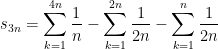
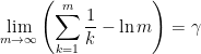
, be the
  th partial sum of this series, so that
  contains
  positive terms with odd denominators and
  .
.
 .
.

 ,
,![s_{3n} = \ln(4n) - \ln 1 + \displaystyle \left( \sum_{k=1}^{4n} \frac{1}{k} - [\ln(4n) - \ln 1]\right)](https://s0.wp.com/latex.php?latex=s_%7B3n%7D+%3D+%5Cln%284n%29+-+%5Cln+1+%2B+%5Cdisplaystyle+%5Cleft%28+%5Csum_%7Bk%3D1%7D%5E%7B4n%7D+%5Cfrac%7B1%7D%7Bk%7D+-+%5B%5Cln%284n%29+-+%5Cln+1%5D%5Cright%29&bg=ffffff&fg=000000&s=0&c=20201002)
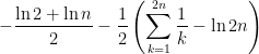
![- \displaystyle \frac{1}{2}[\ln (2n) - \ln 1] - \displaystyle \frac{1}{2} \left( \sum_{k=1}^{2n} \frac{1}{k} - [\ln (2n) - \ln 1]\right)](https://s0.wp.com/latex.php?latex=-+%5Cdisplaystyle+%5Cfrac%7B1%7D%7B2%7D%5B%5Cln+%282n%29+-+%5Cln+1%5D+-+%5Cdisplaystyle+%5Cfrac%7B1%7D%7B2%7D+%5Cleft%28+%5Csum_%7Bk%3D1%7D%5E%7B2n%7D+%5Cfrac%7B1%7D%7Bk%7D+-+%5B%5Cln+%282n%29+-+%5Cln+1%5D%5Cright%29&bg=ffffff&fg=000000&s=0&c=20201002)
![- \displaystyle \frac{1}{2}[\ln n - \ln 1] - \displaystyle \frac{1}{2} \left( \sum_{k=1}^{n} \frac{1}{k} - [\ln n - \ln 1]\right)](https://s0.wp.com/latex.php?latex=-+%5Cdisplaystyle+%5Cfrac%7B1%7D%7B2%7D%5B%5Cln+n+-+%5Cln+1%5D+-+%5Cdisplaystyle+%5Cfrac%7B1%7D%7B2%7D+%5Cleft%28+%5Csum_%7Bk%3D1%7D%5E%7Bn%7D+%5Cfrac%7B1%7D%7Bk%7D+-+%5B%5Cln+n+-+%5Cln+1%5D%5Cright%29&bg=ffffff&fg=000000&s=0&c=20201002)
 ,
,  , and
, and  , we have
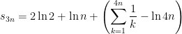
 ,
, .
. :
: .
. ,
,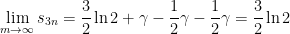 ,
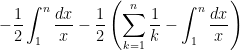
, . For the other partial sums, I note that
 .
.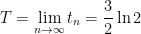 ,
, .
.