In my capstone class for future secondary math teachers, I ask my students to come up with ideas for engaging their students with different topics in the secondary mathematics curriculum. In other words, the point of the assignment was not to devise a full-blown lesson plan on this topic. Instead, I asked my students to think about three different ways of getting their students interested in the topic in the first place.
I plan to share some of the best of these ideas on this blog (after asking my students’ permission, of course).
This student submission comes from my former student Loc Nguyen. His topic, from Precalculus: introducing the number 

How could you as a teacher create an activity or project that involves your topic?
To be able to understand where the number e is produced in the first place, students need to understand how compound interest is calculated. Before introducing the number e, I will definitely create an activity for the students to work on so that they can eventually find the formula for compounding interest based on the patterns they produce throughout the process. The compound interest formula is F=P(1+r/n)nt. From this formula, I will again provide students a worksheet to work on. In this worksheet, I will let P=1, r=100%, t=1, then the compound interest formula will be F=(1+1/n)n. Now students will compute the final value from yearly to secondly.

When they do all the computation, they will see all the decimal places of the final value lining up as n gets big. And finally, they will see that the final value gets to the fixed value as n goes to infinity. That number is e=2.71828162….,
How has this topic appeared in the news?
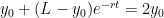
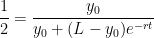
To help the students realize how important number e is, I would engage them with the real life examples or applications. There were some news that incorporated exponential curves. First, I will show the students the news about how fast deadly disease Ebola will grow through this link http://www.npr.org/sections/goatsandsoda/2014/09/18/349341606/why-the-math-of-the-ebola-epidemic-is-so-scary. The students will eventually see how exponential curve comes into play. After that I will provide them this link, http://cleantechnica.com/2014/07/22/exponential-growth-global-solar-pv-production-installation/, in this link, the article talked about the global population rate and it provided the scientific evidence that showed the data collected represent the exponential curve. Up to this point, I will show the students that the population growth model is:

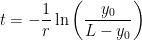
Those examples above was about the growth. For the next example, I will ask the students that how the scientists figured out the age of the earth. In this link, http://earthsky.org/earth/how-old-is-the-earth, the students will learn that the scientists used Modern radiometric dating methods to calculate the age of earth. At this time, I will show them radioactive decay formula and explain to them that this formula is used to determine the lives of the substances such as rocks:
How can technology (YouTube, Khan Academy [khanacademy.org], Vi Hart, Geometers Sketchpad, graphing calculators, etc.) be used to effectively engage students with this topic?
To introduce to the students what the number e is, I will engage them with two videos. In the first video, https://www.youtube.com/watch?v=UFgod5tmLYY, the math song “e a magic number” will engage the students why it is a magic number. While watching this clip, the students will be able to learn the history of e. Also the students will see many mathematical formulas and expressions that contain e. This will give them a heads up that they will see these in future when they take higher level math. It is also pretty humorous of how Dr. Chris Tisdell sang the song.
In the second video, https://www.youtube.com/watch?v=b-MZumdfbt8, it explained why e is everywhere. The video used probability and exponential function to illustrate the usefulness of e, and showed how e is involving in everything. It gave many examples of e such as population, finance… Also the video illustrates the characteristics of the number e and the function that has e in it. Watching these videos will enhance students’ perception and understanding on the number e, and help them to see how important this number is.
Reference
https://www.youtube.com/watch?v=b-MZumdfbt8
https://www.youtube.com/watch?v=UFgod5tmLYY
http://www.math.unt.edu/~baf0018/courses/handouts/exponentialnotes.pdf
http://cleantechnica.com/2014/07/22/exponential-growth-global-solar-pv-production-installation/
http://earthsky.org/earth/how-old-is-the-earth

 .
. and also Taylor series.
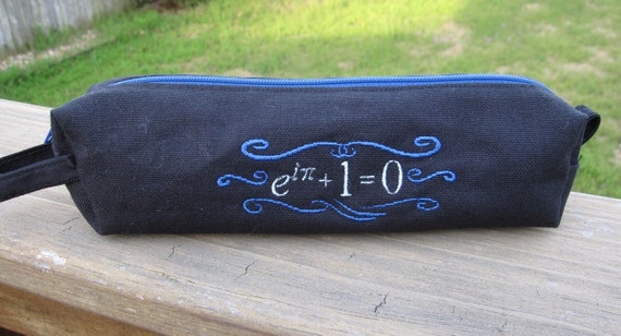


 . The number
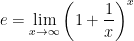
 satisfies the horizontal line test for any
  or
or  . For example,
 ,
, is
is
 and
and  , with
  in the appropriate quadrant. This is analogous to converting from rectangular coordinates to polar coordinates.
 in the case that
  is a complex number.
 be a complex number so that
  . Then we define
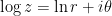 .
. . However, this complex logarithm doesn’t always work the way you’d think it work. For example,
 .
.
 .
.![\log \left[ (-1) \cdot (-1) \right] = \log 1 = 0](https://s0.wp.com/latex.php?latex=%5Clog+%5Cleft%5B+%28-1%29+%5Ccdot+%28-1%29+%5Cright%5D+%3D+%5Clog+1+%3D+0&bg=ffffff&fg=000000&s=0&c=20201002) ,
, .
.
 .
. intercept:
 .
. represents the initial number of people who have the infection.
 gets large:
 .
. people will get the infection eventually. (Of course, Precalculus students won’t be familiar with the $\displaystyle \lim$ notation, but they should understand that
  decays to zero as
  above, it would be a somewhat daunting exercise!
![A' = r A [ L - A] = r L A - r A^2](https://s0.wp.com/latex.php?latex=A%27+%3D+r+A+%5B+L+-+A%5D+%3D+r+L+A+-+r+A%5E2&bg=ffffff&fg=000000&s=0&c=20201002)
 and
and 

 or else
  . The first case corresponds to the trivial cases
  and
and  ; these constants are called the equilibrium solutions. The second case is the more interesting one:

 and solving for
 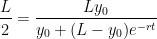 .
. .
.