In this series of posts, we have seen that the number can be thought about in three different ways.

1. defines a region of area 1 under the hyperbola .2. We have the limits

.

These limits form the logical basis for the continuous compound interest formula.

3. We have also shown that . From this derivative, the Taylor series expansion for about can be computed:

Therefore, we can let to find :

In yesterday’s post, I showed that using the original definition (in terms of an area under a hyperbola) does not lend itself well to numerically approximating . Let’s now look at the other two methods.

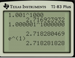
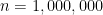
2. The limit gives a somewhat more tractable way of approximating , at least with a modern calculator. However, you can probably imagine the fun of trying to use this formula without a calculator.

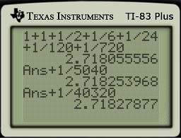
3. The best way to compute (or, in general, ) is with Taylor series. The fractions get very small very quickly, leading to rapid convergence. Indeed, with only terms up to , this approximation beats the above approximation with . Adding just two extra terms comes close to matching the accuracy of the above limit when .

More about approximating via Taylor series can be found in my previous post.