At long last, we have reached the end of this series of posts.
The derivation is elementary; I’m confident that I could have understood this derivation had I seen it when I was in high school. That said, the word “elementary” in mathematics can be a bit loaded — this means that it is based on simple ideas that are perhaps used in a profound and surprising way. Perhaps my favorite quote along these lines was this understated gem from the book Three Pearls of Number Theory after the conclusion of a very complicated proof in Chapter 1:
You see how complicated an entirely elementary construction can sometimes be. And yet this is not an extreme case; in the next chapter you will encounter just as elementary a construction which is considerably more complicated.
Here are the elementary ideas from calculus, precalculus, and high school physics that were used in this series:
- Physics
- Conservation of angular momentum
- Newton’s Second Law
- Newton’s Law of Gravitation
- Precalculus
- Completing the square
- Quadratic formula
- Factoring polynomials
- Complex roots of polynomials
- Bounds on
and
- Period of
- Zeroes of
- Trigonometric identities (Pythagorean, sum and difference, double-angle)
- Conic sections
- Graphing in polar coordinates
- Two-dimensional vectors
- Dot products of two-dimensional vectors (especially perpendicular vectors)
- Euler’s equation
- Calculus
- The Chain Rule
- Derivatives of
- Linearizations of
,
, and
near
(or, more generally, their Taylor series approximations)
- Derivative of
- Solving initial-value problems
- Integration by
substitution


While these ideas from calculus are elementary, they were certainly used in clever and unusual ways throughout the derivation.
I should add that although the derivation was elementary, certain parts of the derivation could be made easier by appealing to standard concepts from differential equations.
One more thought. While this series of post was inspired by a calculation that appeared in an undergraduate physics textbook, I had thought that this series might be worthy of publication in a mathematical journal as an historical example of an important problem that can be solved by elementary tools. Unfortunately for me, Hieu D. Nguyen’s terrific article Rearing Its Ugly Head: The Cosmological Constant and Newton’s Greatest Blunder in The American Mathematical Monthly is already in the record.

 th order homogeneous differential equation with constant coefficients
 ,
,
 determines the solutions of the differential equation.
 . Differentiating, we find
  ,
,  , etc. Therefore, the differential equation becomes


 can never be equal to
  . Therefore, solving the differential equation reduces to finding the roots of this polynomial, which can be done using standard techniques from Precalculus.
 . The characteristic equation is
  , which has roots
  . Therefore, two solutions to the differential equation are
  and
and  , so that the general solution is
 .
. , so that


 .
. . To find the roots of the characteristic equation, we factor:


 .
. , and
, and  , so that the general solution is
 .
. .
.
 and performed a substitution. However, as I’ve discussed in this series, there are four different ways that this integral can be evaluated.
 is independent of
  , I can substitute any convenient value of
  yields the following simplification:


 ,
,  , and
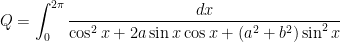
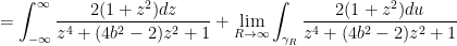
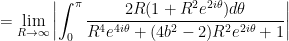
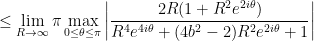
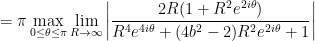
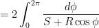
, and  . Now, I’ll calculate this same integral using contour integration. (See
  It turns out that
  ,
, is the contour in the complex plane shown above (graphic courtesy of Mathworld). That’s because


 , so that
  :
:

 .
. while the denominator grows like
  . (This can be more laboriously established using L’Hopital’s rule).
 and then employing the substitution
  (after using trig identities to adjust the limits of integration).
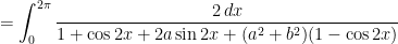


 ,
, and
and 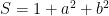 (and
(and  is a certain angle that is now irrelevant at this point in the calculation).
 to evaluate this last integral. Now, I’ll instead use contour integration; see
  ,
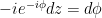
,![\cos \phi = \displaystyle \frac{1}{2} \left[z + \displaystyle \frac{1}{z} \right]](https://s0.wp.com/latex.php?latex=%5Ccos+%5Cphi+%3D+%5Cdisplaystyle+%5Cfrac%7B1%7D%7B2%7D+%5Cleft%5Bz+%2B+%5Cdisplaystyle+%5Cfrac%7B1%7D%7Bz%7D+%5Cright%5D&bg=ffffff&fg=000000&s=0&c=20201002)

 to a the unit circle
  , a closed counterclockwise contour in the complex plane:
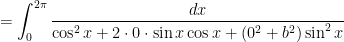
![Q = 2 \displaystyle \oint_C \frac{\displaystyle -\frac{i}{z} dz}{S + \displaystyle \frac{R}{2} \left[z + \displaystyle \frac{1}{z} \right]}](https://s0.wp.com/latex.php?latex=Q+%3D+2+%5Cdisplaystyle+%5Coint_C+%5Cfrac%7B%5Cdisplaystyle+-%5Cfrac%7Bi%7D%7Bz%7D+dz%7D%7BS+%2B+%5Cdisplaystyle+%5Cfrac%7BR%7D%7B2%7D+%5Cleft%5Bz+%2B+%5Cdisplaystyle+%5Cfrac%7B1%7D%7Bz%7D+%5Cright%5D%7D&bg=ffffff&fg=000000&s=0&c=20201002)


 and
and  in terms of
  and
and  . I’ll begin with

![\displaystyle \frac{1}{2} \left[z + \displaystyle \frac{1}{z} \right] = \cos \phi](https://s0.wp.com/latex.php?latex=%5Cdisplaystyle+%5Cfrac%7B1%7D%7B2%7D+%5Cleft%5Bz+%2B+%5Cdisplaystyle+%5Cfrac%7B1%7D%7Bz%7D+%5Cright%5D+%3D+%5Ccos+%5Cphi&bg=ffffff&fg=000000&s=0&c=20201002)
![z - \displaystyle \frac{1}{z} = \cos \phi + i \sin \phi - [ \cos \phi - i \sin \phi]](https://s0.wp.com/latex.php?latex=z+-+%5Cdisplaystyle+%5Cfrac%7B1%7D%7Bz%7D+%3D+%5Ccos+%5Cphi+%2B+i+%5Csin+%5Cphi+-+%5B+%5Ccos+%5Cphi+-+i+%5Csin+%5Cphi%5D&bg=ffffff&fg=000000&s=0&c=20201002)

![\displaystyle \frac{1}{2i} \left[z - \displaystyle \frac{1}{z} \right] = \sin\phi](https://s0.wp.com/latex.php?latex=%5Cdisplaystyle+%5Cfrac%7B1%7D%7B2i%7D+%5Cleft%5Bz+-+%5Cdisplaystyle+%5Cfrac%7B1%7D%7Bz%7D+%5Cright%5D+%3D+%5Csin%5Cphi&bg=ffffff&fg=000000&s=0&c=20201002)
 :
: