At long last, we have reached the end of this series of posts.
The derivation is elementary; I’m confident that I could have understood this derivation had I seen it when I was in high school. That said, the word “elementary” in mathematics can be a bit loaded — this means that it is based on simple ideas that are perhaps used in a profound and surprising way. Perhaps my favorite quote along these lines was this understated gem from the book Three Pearls of Number Theory after the conclusion of a very complicated proof in Chapter 1:
You see how complicated an entirely elementary construction can sometimes be. And yet this is not an extreme case; in the next chapter you will encounter just as elementary a construction which is considerably more complicated.
Here are the elementary ideas from calculus, precalculus, and high school physics that were used in this series:
Physics
Conservation of angular momentum
Newton’s Second Law
Newton’s Law of Gravitation
Precalculus
Completing the square
Quadratic formula
Factoring polynomials
Complex roots of polynomials
Bounds on and
Period of and
Zeroes of and
Trigonometric identities (Pythagorean, sum and difference, double-angle)
Conic sections
Graphing in polar coordinates
Two-dimensional vectors
Dot products of two-dimensional vectors (especially perpendicular vectors)
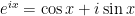
Euler’s equation
Calculus
The Chain Rule
Derivatives of and
Linearizations of , , and near (or, more generally, their Taylor series approximations)
Derivative of
Solving initial-value problems
Integration by substitution
While these ideas from calculus are elementary, they were certainly used in clever and unusual ways throughout the derivation.
I should add that although the derivation was elementary, certain parts of the derivation could be made easier by appealing to standard concepts from differential equations.
One more thought. While this series of post was inspired by a calculation that appeared in an undergraduate physics textbook, I had thought that this series might be worthy of publication in a mathematical journal as an historical example of an important problem that can be solved by elementary tools. Unfortunately for me, Hieu D. Nguyen’s terrific article Rearing Its Ugly Head: The Cosmological Constant and Newton’s Greatest Blunder in The American Mathematical Monthly is already in the record.
In this series, I’m discussing how ideas from calculus and precalculus (with a touch of differential equations) can predict the precession in Mercury’s orbit and thus confirm Einstein’s theory of general relativity. The origins of this series came from a class project that I assigned to my Differential Equations students maybe 20 years ago.
Under general relativity, the motion of a planet around the Sun —in polar coordinates , with the Sun at the origin — satisfies the initial-value problem
,
,
,
where , , , is the gravitational constant of the universe, is the mass of the planet, is the mass of the Sun, is the constant angular momentum of the planet, is the speed of light, and is the smallest distance of the planet from the Sun during its orbit (i.e., at perihelion).
We now take the perspective of a student who is taking a first-semester course in differential equations. There are two standard techniques for solving a second-order non-homogeneous differential equations with constant coefficients. One of these is the method of variation of parameters. First, we solve the associated homogeneous differential equation
.
The characteristic equation of this differential equation is , which clearly has the two imaginary roots . Therefore, two linearly independent solutions of the associated homogeneous equation are and .
(As an aside, this is one answer to the common question, “What are complex numbers good for?” The answer is naturally above the heads of Algebra II students when they first encounter the mysterious number , but complex numbers provide a way of solving the differential equations that model multiple problems in statics and dynamics.)
According to the method of variation of parameters, the general solution of the original nonhomogeneous differential equation
is
,
where
,
,
and is the Wronskian of and , defined by the determinant
.
Well, that’s a mouthful.
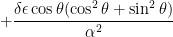
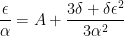
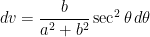
The only good news is that is easy to compute. Since and , we have
from the usual Pythagorean trigonometric identity. Therefore, the denominators in the integrals for and essentially disappear.
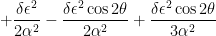
Unfortunately, computing and , using
,
is a beast, requiring the creative use of multiple trigonometric identities. We begin with , using the substitution :
,
where we use for the constant of integration instead of the usual . Second,
.
Unfortunately, this is not easily simplified with a substitution, so we have to expand the integrand:
,
using for the constant of integration. Therefore, by variation of parameters, the general solution of the nonhomogeneous differential equation is
,
where is another arbitrary constant.
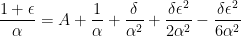
Next, we use the initial conditions to find the constants and . From the initial condition , we obtain
,
so that
.
Next, we compute and use the initial condition :
.
Substituting these values for and , we finally arrive at the solution
In this series, I’m discussing how ideas from calculus and precalculus (with a touch of differential equations) can predict the precession in Mercury’s orbit and thus confirm Einstein’s theory of general relativity. The origins of this series came from a class project that I assigned to my Differential Equations students maybe 20 years ago.
In the last post, we showed that if the motion of a planet around the Sun is expressed in polar coordinates , with the Sun at the origin, then under general relativity the motion of the planet follows the initial-value problem
,
,
,
where , , , is the gravitational constant of the universe, is the mass of the planet, is the mass of the Sun, is the constant angular momentum of the planet, is the speed of light, and is the smallest distance of the planet from the Sun during its orbit (i.e., at perihelion).
I won’t sugar-coat it; the solution is a big mess:
.
That said, it is an elementary, if complicated, exercise in calculus to confirm that this satisfies all three equations above. We’ll start with the second one:
,
where in the last step we used the equation that was obtained earlier in this series.
Next, to check the initial condition , we differentiate:
.
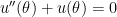
Finally, to check the differential equation itself, we compute the second derivative:
.
Adding and , we find
,
which simplifies considerably:
,
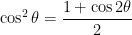
where we used the power-reduction trigonometric identity
on the second-to-last step.
While we have verified the proposed solution of the initial-value problem, and the steps for doing so lie completely within the grasp of a good calculus student, I’ll be the first to say that this solution is somewhat unsatisfying: the solution appeared seemingly out of thin air, and we just checked to see if this mysterious solution actually works. In the next few posts, I’ll discuss how this solution can be derived using standard techniques from first-semester differential equations.
The proofs of Kepler’s Three Laws are usually included in textbooks for multivariable calculus. So I was very intrigued when I saw, in the Media Reviews of College Mathematics Journal, that somebody had published a proof of Kepler’s First Law that only uses algebra and trigonometry. Let me quote from the review:
Kepler’s first law states that bounded planetary orbits are elliptical. This law is presented in introductory textbooks, but the proof typically requires intricate integrals or vector analysis involving an accidental degeneracy. Simha offers an elementary proof of Kepler’s first law using algebra and trigonometry at the high school level.
Once upon a time, I taught Precalculus for precocious high school students. I wish I had known of this result back then, as it would have been a wonderful capstone to their studies of trigonometry and the conic sections.
The preprint of this result can be found on arXiv. (The proof only addresses Kepler’s First Law and not the Second and Third Laws.) The actual article, for those with institutional access, was published in American Journal of Physics Vol. 89 No. 11 (2021): 1009-1011.
In my capstone class for future secondary math teachers, I ask my students to come up with ideas for engaging their students with different topics in the secondary mathematics curriculum. In other words, the point of the assignment was not to devise a full-blown lesson plan on this topic. Instead, I asked my students to think about three different ways of getting their students interested in the topic in the first place.
I plan to share some of the best of these ideas on this blog (after asking my students’ permission, of course).
This student submission comes from my former student Morgan Mayfield. His topic, from Precalculus: deriving the double angle formulas for sine, cosine, and tangent.
How could you as a teacher create an activity or project that involves your topic?
I want to provide some variety for opportunities to make this an engaging opportunity for Precalculus students and some Calculus students. Here are my three thoughts:
IDEA 1:
For precalculus students in a regular or advanced class, have them derive this formula in groups. After students are familiar with the Pythagorean identities and with angle sum identities, group students and ask them to derive a formula for double angles Sin(2θ), Cos(2θ), Tan(2θ). Let them struggle a bit, and if needed give them some hints such as useful formulas and ways to represent multiplication so that it looks like other operations. From here, encourage students to simplify when they can and challenge students to find the other formulas of Cos(2θ). Ask students to speculate instances when each formula for Cos(2θ) would be advantageous. This gives students confidence in their own abilities and show how math is interconnected and not just a bunch of trivial formulas.
Lastly, to challenge students, have them come up with an alternative way to prove Tan(2θ), notably Sin(2θ)/Cos(2θ). This would make an appropriate activity for students while having them continue practicing proving trigonometric identities.
IDEA 2:
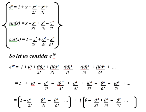
This next idea should be implemented for an advanced Precal class, and only when there is some time to spare. Euler was an intelligent man and left us with the Euler’s Formula: . Have Precalculus students suspend their questions about where it comes from and what it is used for. This is not something they would use in their class. Reassure them that for what they will do, all they need to understand is imaginary numbers, multiplying imaginary numbers, and laws of exponents. Have them plug in x = A + B and simplify the right-hand side of the equation so that we get: where and are two real numbers. The goal here is to get . All the steps to get to this point is Algebra, nothing out of their grasp. Now, the next part is to really get their brains going about what meaning we can make of this. If they are struggling, have them think about the implications of two imaginary numbers being equal; the coefficient of the real parts and imaginary parts must be equal to each other. Lastly, ask them if these equations seem familiar, where are they from, and what are they called…the angle sum formulas. From here, this can lead into what if x=2A? Students will either brute force the formula again, and others will realize x = A + A and plug it in to the equation they just derived and simplify. This idea is a 2-in-1 steal for the angle sum formulas and double angle formulas. It’s biggest downside is this is for Sin(2θ) and Cos(2θ).IDEA 3:
Take IDEA 2, and put it in a Calculus 2 class. Everything that the precalculus class remains, but now have the paired students prove the Euler’s Formula using Taylor Series. Guide them through using the Taylor Series to figure out a Taylor Series representation of , , and . Then ask students to find an expanded Taylor Series of to 12 terms with ellipses, no need to evaluate each term, just the precise term. Give hints such as and to consider and other similar cases. Lastly, ask students to separate the extended series in a way that mimics using ellipses to shows the series goes to infinity. What they should find is something like this:
Look familiar? Well it is the addition of two Taylor Series that represent Sin(x) and Cos(x). This is the last connection students need to make. Give hints to look through their notes to see why the “a” and “b” in the imaginary number look so familiar. This, is just one way to prove Euler’s Formula, then you can continue with IDEA 2 until your students prove the angle sum formulas and double angle formulas.
How does this topic extend what your students should have learned in previous courses?
Students in Texas will typically be exposed to the Pythagorean Theorem in 8th grade. At this stage, students use to find a missing side length. Students may also be exposed to Pythagorean triples at this stage. Then at the Geometry level or in a Trigonometry section, students will be exposed to the Pythagorean Identity. The Identity is . I think that this is not fair for students to just learn this identity without connecting it to the Pythagorean Theorem. I think it would be a nice challenge student to solve for this identity by using a right triangle with hypotenuse c so that Sin (θ) = b/c and cos (θ) = a/c, one could then show either and thus or one could show (using the Pythagorean theorem).
From here, students learn about the angle addition and subtraction formulas in Precalculus. This is all that they need to derive the double angle formulas.
This would be a good challenge exercise for students to do in pairs. Sin(2θ) = Sin(θ + θ), Cos(2 θ) = Cos(θ + θ), Tan(2θ) = Tan(θ + θ). Now we can apply the angle sum formula where both angles are equal:
Sin(2θ) = sin(θ)cos(θ) + cos(θ)sin(θ) = 2sin(θ)cos(θ)
Cos(2θ) = cos(θ)cos(θ) – sin(θ)sin(θ) = (We use a Pythagorean Identity here)
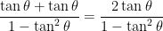
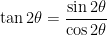
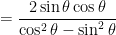
Tan(2θ) =
Bonus challenge, use Sin(2θ) and Cos(2θ) to get Tan(2θ). Well, if , then
The derivations are straight forward, and I believe that many students get off the hook by not being exposed to deriving many trigonometric identities and taking them as facts. This is in the grasp of an average 10th to 12th grader.
What are the contributions of various cultures to this topic?
I have included four links that talk about the history of Trigonometry. It seemed that ancient societies would need to know about the Pythagorean Identities and the angles sum formulas to know the double angle formulas. Here is our problem, it’s hard to know who “did it first?” and when “did they know it?”. Mathematical proofs and history were not kept as neatly written record but as oral traditions, entertainment, hobbies, and professions. The truth is that from my reading, many cultures understood the double angle formula to some extent independently of each other, even if there was no formal proof or record of it. Looking back at my answer to B2, it seems that the double angle formula is almost like a corollary to knowing the angle sum formulas, and thus to understand one could imply knowledge of the other. Perhaps, it was just not deemed important to put the double angle formula into a category of its own. Many of the people who figured out these identities were doing it because they were astronomers, navigators, or carpenters (construction). Triangles and circles are very important to these professions. Knowledge of the angle sum formula was known in Ancient China, Ancient India, Egypt, Greece (originally in the form of broken chords theorem by Archimedes), and the wider “Medieval Islamic World”. Do note that that Egypt, Greece, and the Medieval Islamic World were heavily intertwined as being on the east side of the Mediterranean and being important centers of knowledge (i.e. Library of Alexandria.) Here is the thing, their knowledge was not always demonstrated in the same way as we know it today. Some cultures did have functions similar to the modern trigonometric functions today, and an Indian mathematician, Mādhava of Sangamagrāma, figured out the Taylor Series approximations of those functions in the 1400’s. Greece and China for example relayed heavily on displaying knowledge of trigonometry in ideas of the length of lines (rods) as manifestations of variables and numbers. Ancient peoples didn’t have calculators, and they may have defined trigonometric functions in a way that would be correct such as the “law of sines” or a “Taylor series”, but still relied on physical “sine tables” to find a numerical representation of sine to n numbers after the decimal point. How we think of Geometry and Trigonometry today may have come from Descartes’ invention of the Cartesian plane as a convenient way to bridge Algebra and Geometry.
References:
https://www.mathpages.com/home/kmath205/kmath205.htmhttps://en.wikipedia.org/wiki/History_of_trigonometryhttps://www.ima.umn.edu/press-room/mumford-and-pythagoras-theorem
In my capstone class for future secondary math teachers, I ask my students to come up with ideas for engaging their students with different topics in the secondary mathematics curriculum. In other words, the point of the assignment was not to devise a full-blown lesson plan on this topic. Instead, I asked my students to think about three different ways of getting their students interested in the topic in the first place.
I plan to share some of the best of these ideas on this blog (after asking my students’ permission, of course).
This student submission comes from my former student Daniel Adkins. His topic, from Precalculus: deriving the double angle formulas for sine, cosine, and tangent.
How does this topic extend what your students should have already learned?
A major factor that simplifies deriving the double angle formulas is recalling the trigonometric identities that help students “skip steps.” This is true especially for the Sum formulas, so a brief review of these formulas in any fashion would help students possibly derive the equations on their own in some cases. Listed below are the formulas that can lead directly to the double angle formulas.
A list of the formulas that students can benefit from recalling:
Sum Formulas:
sin(a+b) = sin(a)cos(b) + cos(a)sin(b)
cos(a+b) = cos(a)cos(b) – sin(a)sin(b)
tan(a+b) = [tan(a) +tan(b)] / [1-tan(a)tan(b)]
Pythagorean Identity:
Sin2 (a) + Cos2(a) = 1
This leads to the next topic, an activity for students to attempt the equation on their own.
How could you as a teacher create an activity or project that involves your topic?
I’m a firm believer that the more often a student can learn something of their own accord, the better off they are. Providing the skeletal structure of the proofs for the double angle formulas of sine, cosine, and tangent might be enough to help students reach the formulas themselves. The major benefit of this is that, even though these are simple proofs, they have a lot of variance on how they may be presented to students and how “hands on” the activity can be.
I have an example worksheet demonstrating this with the first two double angle formulas attached below. This is in extremely hands on format that can be given to students with the formulas needed in the top right corner and the general position where these should be inserted. If needed the instructor could take this a step further and have the different Pythagorean Identities already listed out (I.e. Cos2(a) = 1 – Sin2(a), Sin2(a) = 1 – Cos2(a)) to emphasize that different formats could be needed. This is an extreme that wouldn’t take students any time to reach the conclusions desired. Of course a lot of this information could be dropped to increase the effort needed to reach the conclusion.
A major benefit with this also is that even though they’re simple, students will still feel extremely rewarded from succeeding on this paper on their own, and thus would be more intrinsically motivated towards learning trig identities.
How can Technology be used to effectively engage students with this topic?
When it comes to technology in the classroom, I tend to lean more on the careful side. I know me as a person/instructor, and I know I can get carried away and make a mess of things because there was so much excitement over a new toy to play with. I also know that the technology can often detract from the actual math itself, but when it comes to trigonometry, and basically any form of geometric mathematics, it’s absolutely necessary to have a visual aid, and this is where technology excels.
The Wolfram Company has provided hundreds of widgets for this exact purpose, and below, you’ll find one attached that demonstrates that sin(2a) appears to be equal to its identity 2cos(a)sin(a). This is clearly not a rigorous proof, but it will help students visualize how these formulas interact with each other and how they may be similar. The fact that it isn’t rigorous may even convince students to try to debunk it. If you can make a student just irritated enough that they spend a few minutes trying to find a way to show you that you’re wrong, then you’ve done your job in that you’ve convinced them to try mathematics for a purpose.
After all, at the end of the day, it doesn’t matter how you begin your classroom, or how you engage your students, what matters is that they are engaged, and are willing to learn.
Some husbands try to impress their wives by lifting extremely heavy objects or other extraordinary feats of physical prowess.
That will never happen in the Quintanilla household in a million years.
But she was impressed that I broke an impasse in her research and resolved a discrepancy between Mathematica 4 and Mathematica 8 by finding the following integral by hand in less than an hour:
Yes, I married well indeed.
In this post, I collect the posts that I wrote last summer regarding various ways of computing this integral.
Part 2a, 2b, 2c, 2d, 2e, 2f: Changing the endpoints of integration, multiplying top and bottom by , and the substitution .
Part 3a, 3b, 3c, 3d, 3e, 3f, 3g, 3h, 3i: Double-angle trig identity, combination into a single trig function, changing the endpoints of integration, and the magic substitution .
Part 4a, 4b, 4c, 4d, 4e, 4f, 4g, 4h: Double-angle trig identity, combination into a single trig function, changing the endpoints of integration, and contour integration using the unit circle
Part 5a, 5b, 5c, 5d, 5e, 5f, 5g, 5h, 5i, 5j: Independence of the parameter , the magic substitution , and partial fractions.
Part 6a, 6b, 6c, 6d, 6e, 6f, 6g:Independence of the parameter , the magic substitution , and contour integration using the real line and an expanding semicircle.
Part 7: Concluding thoughts… and ways that should work that I haven’t completely figured out yet.
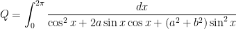
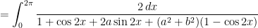
Earlier in this series, I gave three different methods of showing that
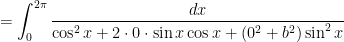
Using the fact that is independent of , I’ll now give a fourth method. Since is independent of , I can substitute any convenient value of that I want without changing the value of . As shown in previous posts, substituting yields the following simplification:
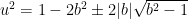
The four roots of the denominator satisfy
So far, I’ve handled the cases and . In today’s post, I’ll start considering the case .
Factoring the denominator is a bit more complicated if . Using the quadratic equation, we obtain
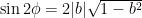
However, unlike the cases , the right-hand side is now a complex number. So, To solve for , I’ll use DeMoivre’s Theorem and some surprisingly convenient trig identities. Notice that
.
Therefore, the four complex roots of the denominator satisfy , or . This means that all four roots can be written in trigonometric form so that
,
where is some angle. (I chose the angle to be instead of for reasons that will become clear shortly.)
I’ll begin with solving
.
Matching the real and imaginary parts, we see that
,
This completely matches the form of the double-angle trig identities
,
,
and so the problem reduces to solving
,
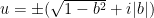
where $\sin \phi = |b|$ and $\cos \phi = \sqrt{1-b^2}$. By De Moivre’s Theorem, I can conclude that the two solutions of this equation are
,
or
.
I could re-run this argument to solve and get the other two complex roots. However, by the Conjugate Root Theorem, I know that the four complex roots of the denominator must come in conjugate pairs. Therefore, the four complex roots are
.
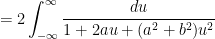
Therefore, I can factor the denominator as follows:
To double-check my work, I can directly multiply this product:
.
So, at last, I can rewrite the integral as
I’ll continue with this fourth evaluation of the integral, continuing the case , in tomorrow’s post.
Amazingly, the integral below has a simple solution:
Even more amazingly, the integral ultimately does not depend on the parameter . For several hours, I tried to figure out a way to demonstrate that is independent of , but I couldn’t figure out a way to do this without substantially simplifying the integral, but I’ve been unable to do so (at least so far).
So here’s what I have been able to develop to prove that is independent of without directly computing the integral .
Earlier in this series, I showed that
Yesterday, I showed used the substitution to show that was independent of . Today, I’ll use a different method to establish the same result. Let
.
Notice that I’ve written this integral as a function of the parameter . I will demonstrate that , so that is a constant with respect to . In other words, does not depend on .
To do this, I differentiate under the integral sign with respect to (as opposed to ) using the Quotient Rule:
I now apply the trigonometric substitution , so that
and
The endpoints of integration change from to , and so
.
I’m not completely thrilled with this demonstration that is independent of , mostly because I had to do so much simplification of the integral to get this result. As I mentioned in yesterday’s post, I’d love to figure out a way to directly start with
and demonstrate that is independent of , perhaps by differentiating with respect to and demonstrating that the resulting integral must be equal to 0. However, despite several hours of trying, I’ve not been able to establish this result without simplifying first.
My wife had asked me to compute this integral by hand because Mathematica 4 and Mathematica 8 gave different answers. At the time, I eventually obtained the solution by multiplying the top and bottom of the integrand by and then employing the substitution (after using trig identities to adjust the limits of integration).
But this wasn’t the only method I tried. Indeed, I tried two or three different methods before deciding they were too messy and trying something different. So, for the rest of this series, I’d like to explore different ways that the above integral can be computed.
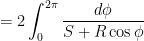
So far, I have shown that
where and (and is a certain angle that is now irrelevant at this point in the calculation).
There are actually a couple of ways for computing this last integral. Today, I’ll lay the foundation for the “magic substitution”
With this substitution, the above integral will become a rational function, which can then be found using standard techniques.
First, we use some trig identities to rewrite in terms of :
Next, I’ll replace by :
.
Second, for the sake of completeness (even though it isn’t necessary for this particular integral), I’ll rewrite in terms of :
Next, I’ll replace by :
.
Third, again for the sake of completeness,
.
Finally, I need to worry about what happens to the :
These four substitutions can be used to convert trigonometric integrals into some other integral. Usually, the new integrand is pretty messy, and so these substitutions should only be used sparingly, as a last resort.
I’ll continue this different method of evaluating this integral in tomorrow’s post.
and
,
, and
near
(or, more generally, their Taylor series approximations)
substitution


 , with the Sun at the origin — satisfies the initial-value problem
 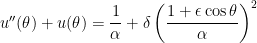 ,
, ,
, ,
, ,
,  ,
,  ,
,  is the gravitational constant of the universe,
  is the mass of the planet,
  is the mass of the Sun,
  is the constant angular momentum of the planet,
  is the speed of light, and
  is the smallest distance of the planet from the Sun during its orbit (i.e., at perihelion).
 .
. , which clearly has the two imaginary roots
  . Therefore, two linearly independent solutions of the associated homogeneous equation are
  and
and  .
. , but complex numbers provide a way of solving the differential equations that model multiple problems in statics and dynamics.)
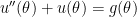
 ,
, ,
, ,
, is the Wronskian of
  and
and  , defined by the determinant
 .
. is easy to compute. Since
 and
and  essentially disappear.
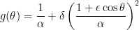 ,
,  :
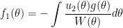
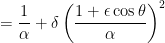
:![f_1(\theta) = -\displaystyle \int \left[ \frac{1}{\alpha} + \delta \left( \frac{1 + \epsilon \cos \theta}{\alpha} \right)^2 \right] \sin \theta \, d\theta](https://s0.wp.com/latex.php?latex=f_1%28%5Ctheta%29+%3D+-%5Cdisplaystyle+%5Cint+%5Cleft%5B+%5Cfrac%7B1%7D%7B%5Calpha%7D+%2B+%5Cdelta+%5Cleft%28+%5Cfrac%7B1+%2B+%5Cepsilon+%5Ccos+%5Ctheta%7D%7B%5Calpha%7D+%5Cright%29%5E2+%5Cright%5D+%5Csin+%5Ctheta+%5C%2C+d%5Ctheta&bg=ffffff&fg=000000&s=0&c=20201002)
![= \displaystyle \int \left[ \frac{1}{\alpha} + \delta \left( \frac{1 + \epsilon t}{\alpha} \right)^2 \right] \, dt](https://s0.wp.com/latex.php?latex=%3D+%5Cdisplaystyle+%5Cint+%5Cleft%5B+%5Cfrac%7B1%7D%7B%5Calpha%7D+%2B+%5Cdelta+%5Cleft%28+%5Cfrac%7B1+%2B+%5Cepsilon+t%7D%7B%5Calpha%7D+%5Cright%29%5E2+%5Cright%5D+%5C%2C+dt&bg=ffffff&fg=000000&s=0&c=20201002)

 ,
, for the constant of integration instead of the usual
  . Second,
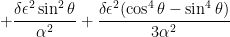
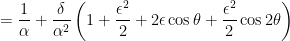
![f_2(\theta) = \displaystyle \int \left[ \frac{1}{\alpha} + \delta \left( \frac{1 + \epsilon \cos \theta}{\alpha} \right)^2 \right] \cos\theta \, d\theta](https://s0.wp.com/latex.php?latex=f_2%28%5Ctheta%29+%3D+%5Cdisplaystyle+%5Cint+%5Cleft%5B+%5Cfrac%7B1%7D%7B%5Calpha%7D+%2B+%5Cdelta+%5Cleft%28+%5Cfrac%7B1+%2B+%5Cepsilon+%5Ccos+%5Ctheta%7D%7B%5Calpha%7D+%5Cright%29%5E2+%5Cright%5D+%5Ccos%5Ctheta+%5C%2C+d%5Ctheta&bg=ffffff&fg=000000&s=0&c=20201002) .
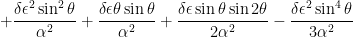
.![f_2(\theta) = \displaystyle \int \left[ \frac{\cos \theta}{\alpha} + \frac{\delta \cos \theta}{\alpha^2} + \frac{2 \delta \epsilon \cos^2 \theta}{\alpha^2} + \frac{\delta \epsilon^2 \cos^3 \theta}{\alpha^2} \right] \, d\theta](https://s0.wp.com/latex.php?latex=f_2%28%5Ctheta%29+%3D+%5Cdisplaystyle+%5Cint+%5Cleft%5B+%5Cfrac%7B%5Ccos+%5Ctheta%7D%7B%5Calpha%7D+%2B+%5Cfrac%7B%5Cdelta+%5Ccos+%5Ctheta%7D%7B%5Calpha%5E2%7D+%2B+%5Cfrac%7B2+%5Cdelta+%5Cepsilon+%5Ccos%5E2+%5Ctheta%7D%7B%5Calpha%5E2%7D+%2B+%5Cfrac%7B%5Cdelta+%5Cepsilon%5E2+%5Ccos%5E3+%5Ctheta%7D%7B%5Calpha%5E2%7D+%5Cright%5D+%5C%2C+d%5Ctheta&bg=ffffff&fg=000000&s=0&c=20201002)
![= \displaystyle \int \left[ \frac{\cos \theta}{\alpha} + \frac{\delta \cos \theta}{\alpha^2} + \frac{\delta \epsilon (1 + \cos 2 \theta)}{\alpha^2} + \frac{\delta \epsilon^2 \cos \theta \cos^2 \theta}{\alpha^2} \right] \, d\theta](https://s0.wp.com/latex.php?latex=%3D+%5Cdisplaystyle+%5Cint+%5Cleft%5B+%5Cfrac%7B%5Ccos+%5Ctheta%7D%7B%5Calpha%7D+%2B+%5Cfrac%7B%5Cdelta+%5Ccos+%5Ctheta%7D%7B%5Calpha%5E2%7D+%2B+%5Cfrac%7B%5Cdelta+%5Cepsilon+%281+%2B+%5Ccos+2+%5Ctheta%29%7D%7B%5Calpha%5E2%7D+%2B+%5Cfrac%7B%5Cdelta+%5Cepsilon%5E2+%5Ccos+%5Ctheta+%5Ccos%5E2+%5Ctheta%7D%7B%5Calpha%5E2%7D+%5Cright%5D+%5C%2C+d%5Ctheta&bg=ffffff&fg=000000&s=0&c=20201002)
![= \displaystyle \int \left[ \frac{\cos \theta}{\alpha} + \frac{\delta \cos \theta}{\alpha^2} + \frac{\delta \epsilon}{\alpha^2} + \frac{\delta \epsilon \cos 2 \theta}{\alpha^2}+ \frac{\delta \epsilon^2 \cos \theta (1- \sin^2 \theta)}{\alpha^2} \right] \, d\theta](https://s0.wp.com/latex.php?latex=%3D+%5Cdisplaystyle+%5Cint+%5Cleft%5B+%5Cfrac%7B%5Ccos+%5Ctheta%7D%7B%5Calpha%7D+%2B+%5Cfrac%7B%5Cdelta+%5Ccos+%5Ctheta%7D%7B%5Calpha%5E2%7D+%2B+%5Cfrac%7B%5Cdelta+%5Cepsilon%7D%7B%5Calpha%5E2%7D+%2B+%5Cfrac%7B%5Cdelta+%5Cepsilon+%5Ccos+2+%5Ctheta%7D%7B%5Calpha%5E2%7D%2B+%5Cfrac%7B%5Cdelta+%5Cepsilon%5E2+%5Ccos+%5Ctheta+%281-+%5Csin%5E2+%5Ctheta%29%7D%7B%5Calpha%5E2%7D+%5Cright%5D+%5C%2C+d%5Ctheta&bg=ffffff&fg=000000&s=0&c=20201002)
![= \displaystyle \int \left[ \frac{\cos \theta}{\alpha} + \frac{\delta (1 + \epsilon^2) \cos \theta}{\alpha^2} + \frac{\delta \epsilon}{\alpha^2} + \frac{\delta \epsilon \cos 2 \theta}{\alpha^2} - \frac{\delta \epsilon^2 \cos \theta \sin^2 \theta}{\alpha^2} \right] \, d\theta](https://s0.wp.com/latex.php?latex=%3D+%5Cdisplaystyle+%5Cint+%5Cleft%5B+%5Cfrac%7B%5Ccos+%5Ctheta%7D%7B%5Calpha%7D+%2B+%5Cfrac%7B%5Cdelta+%281+%2B+%5Cepsilon%5E2%29+%5Ccos+%5Ctheta%7D%7B%5Calpha%5E2%7D++%2B+%5Cfrac%7B%5Cdelta+%5Cepsilon%7D%7B%5Calpha%5E2%7D+%2B+%5Cfrac%7B%5Cdelta+%5Cepsilon+%5Ccos+2+%5Ctheta%7D%7B%5Calpha%5E2%7D+-+%5Cfrac%7B%5Cdelta+%5Cepsilon%5E2+%5Ccos+%5Ctheta+%5Csin%5E2+%5Ctheta%7D%7B%5Calpha%5E2%7D+%5Cright%5D+%5C%2C+d%5Ctheta&bg=ffffff&fg=000000&s=0&c=20201002)
 ,
, for the constant of integration. Therefore, by variation of parameters, the general solution of the nonhomogeneous differential equation is
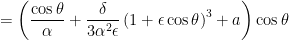


 ,
, is another arbitrary constant.
 . From the initial condition
  , we obtain
 ,
, .
. and use the initial condition

 .
.
 .
. .
.


 ,
, that was obtained earlier in this series.
 .
. .
. and
and  , we find
 ,
,
 ,
,
 . Have Precalculus students suspend their questions about where it comes from and what it is used for. This is not something they would use in their class. Reassure them that for what they will do, all they need to understand is imaginary numbers, multiplying imaginary numbers, and laws of exponents. Have them plug in x = A + B and simplify the right-hand side of the equation so that we get:
  where
where  and
and  . All the steps to get to this point is Algebra, nothing out of their grasp. Now, the next part is to really get their brains going about what meaning we can make of this. If they are struggling, have them think about the implications of two imaginary numbers being equal; the coefficient of the real parts and imaginary parts must be equal to each other. Lastly, ask them if these equations seem familiar, where are they from, and what are they called…the angle sum formulas. From here, this can lead into what if x=2A? Students will either brute force the formula again, and others will realize x = A + A and plug it in to the equation they just derived and simplify. This idea is a 2-in-1 steal for the angle sum formulas and double angle formulas. It’s biggest downside is this is for Sin(2θ) and Cos(2θ).
IDEA 3:
Take IDEA 2, and put it in a Calculus 2 class. Everything that the precalculus class remains, but now have the paired students prove the Euler’s Formula using Taylor Series. Guide them through using the Taylor Series to figure out a Taylor Series representation of
. All the steps to get to this point is Algebra, nothing out of their grasp. Now, the next part is to really get their brains going about what meaning we can make of this. If they are struggling, have them think about the implications of two imaginary numbers being equal; the coefficient of the real parts and imaginary parts must be equal to each other. Lastly, ask them if these equations seem familiar, where are they from, and what are they called…the angle sum formulas. From here, this can lead into what if x=2A? Students will either brute force the formula again, and others will realize x = A + A and plug it in to the equation they just derived and simplify. This idea is a 2-in-1 steal for the angle sum formulas and double angle formulas. It’s biggest downside is this is for Sin(2θ) and Cos(2θ).
IDEA 3:
Take IDEA 2, and put it in a Calculus 2 class. Everything that the precalculus class remains, but now have the paired students prove the Euler’s Formula using Taylor Series. Guide them through using the Taylor Series to figure out a Taylor Series representation of  , and
, and  . Then ask students to find an expanded Taylor Series of to 12 terms with ellipses, no need to evaluate each term, just the precise term. Give hints such as
  and to consider
  and other similar cases. Lastly, ask students to separate the extended series in a way that mimics
  using ellipses to shows the series goes to infinity. What they should find is something like this:
 to find a missing side length. Students may also be exposed to Pythagorean triples at this stage. Then at the Geometry level or in a Trigonometry section, students will be exposed to the Pythagorean Identity. The Identity is
 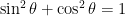 . I think that this is not fair for students to just learn this identity without connecting it to the Pythagorean Theorem. I think it would be a nice challenge student to solve for this identity by using a right triangle with hypotenuse c so that Sin (θ) = b/c and cos (θ) = a/c, one could then show either
  and thus
  or one could show
  (using the Pythagorean theorem).
From here, students learn about the angle addition and subtraction formulas in Precalculus. This is all that they need to derive the double angle formulas.
(using the Pythagorean theorem).
From here, students learn about the angle addition and subtraction formulas in Precalculus. This is all that they need to derive the double angle formulas.


 Bonus challenge, use Sin(2θ) and Cos(2θ) to get Tan(2θ). Well, if
  , then


 , and the substitution
  .
. .
.
 is independent of
  yields the following simplification:


 and
and  . In today’s post, I’ll start considering the case
  .
.
 , the right-hand side is now a complex number. So, To solve for
  , I’ll use
  .
. , or
, or  . This means that all four roots can be written in
 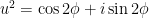 ,
, is some angle. (I chose the angle to be
  for reasons that will become clear shortly.)
 .
. ,
,
 ,
, ,
, ,
, .
. and get the other two complex roots. However, by the Conjugate Root Theorem, I know that the four complex roots of the denominator
  must come in conjugate pairs. Therefore, the four complex roots are
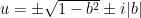 .
.![u^4 + (4 b^2 - 2) u^2 + 1 = (u - [\sqrt{1-b^2} + i|b|])(u - [\sqrt{1-b^2} - i|b|])](https://s0.wp.com/latex.php?latex=u%5E4+%2B+%284+b%5E2+-+2%29+u%5E2+%2B+1+%3D+%28u+-+%5B%5Csqrt%7B1-b%5E2%7D+%2B+i%7Cb%7C%5D%29%28u+-+%5B%5Csqrt%7B1-b%5E2%7D+-+i%7Cb%7C%5D%29&bg=ffffff&fg=000000&s=0&c=20201002)
![\qquad \times (u - [-\sqrt{1-b^2} + i|b|])(u - [-\sqrt{1-b^2} + i|b|])](https://s0.wp.com/latex.php?latex=%5Cqquad+%5Ctimes+%28u+-+%5B-%5Csqrt%7B1-b%5E2%7D+%2B+i%7Cb%7C%5D%29%28u+-+%5B-%5Csqrt%7B1-b%5E2%7D+%2B+i%7Cb%7C%5D%29&bg=ffffff&fg=000000&s=0&c=20201002)
![= (u - \sqrt{1-b^2} - i|b|)(u - \sqrt{1-b^2} + i|b])](https://s0.wp.com/latex.php?latex=%3D+%28u+-+%5Csqrt%7B1-b%5E2%7D+-+i%7Cb%7C%29%28u+-+%5Csqrt%7B1-b%5E2%7D+%2B+i%7Cb%5D%29&bg=ffffff&fg=000000&s=0&c=20201002)

![= ([u - \sqrt{1-b^2}]^2 +b^2)([u + \sqrt{1-b^2}]^2 +b^2)](https://s0.wp.com/latex.php?latex=%3D+%28%5Bu+-+%5Csqrt%7B1-b%5E2%7D%5D%5E2+%2Bb%5E2%29%28%5Bu+%2B+%5Csqrt%7B1-b%5E2%7D%5D%5E2+%2Bb%5E2%29&bg=ffffff&fg=000000&s=0&c=20201002)
![([u - \sqrt{1-b^2}]^2 +b^2)([u + \sqrt{1-b^2}]^2 +b^2)](https://s0.wp.com/latex.php?latex=%28%5Bu+-+%5Csqrt%7B1-b%5E2%7D%5D%5E2+%2Bb%5E2%29%28%5Bu+%2B+%5Csqrt%7B1-b%5E2%7D%5D%5E2+%2Bb%5E2%29&bg=ffffff&fg=000000&s=0&c=20201002)

![= ([u^2 +1] - 2u\sqrt{1-b^2})([u^2+1] + 2u\sqrt{1-b^2})](https://s0.wp.com/latex.php?latex=%3D+%28%5Bu%5E2+%2B1%5D+-+2u%5Csqrt%7B1-b%5E2%7D%29%28%5Bu%5E2%2B1%5D+%2B+2u%5Csqrt%7B1-b%5E2%7D%29&bg=ffffff&fg=000000&s=0&c=20201002)
![= [u^2+1]^2 - [2u\sqrt{1-b^2}]^2](https://s0.wp.com/latex.php?latex=%3D+%5Bu%5E2%2B1%5D%5E2+-+%5B2u%5Csqrt%7B1-b%5E2%7D%5D%5E2&bg=ffffff&fg=000000&s=0&c=20201002)

![= u^4 + u^2 (2 - 4[1-b^2]) + 1](https://s0.wp.com/latex.php?latex=%3D+u%5E4+%2B+u%5E2+%282+-+4%5B1-b%5E2%5D%29+%2B+1&bg=ffffff&fg=000000&s=0&c=20201002)
 .
.![Q = \displaystyle \int_{-\infty}^{\infty} \frac{ 2(1+u^2) du}{ ([u - \sqrt{1-b^2}]^2 +b^2)([u + \sqrt{1-b^2}]^2 +b^2)}](https://s0.wp.com/latex.php?latex=Q+%3D+%5Cdisplaystyle+%5Cint_%7B-%5Cinfty%7D%5E%7B%5Cinfty%7D+%5Cfrac%7B+2%281%2Bu%5E2%29+du%7D%7B+%28%5Bu+-+%5Csqrt%7B1-b%5E2%7D%5D%5E2+%2Bb%5E2%29%28%5Bu+%2B+%5Csqrt%7B1-b%5E2%7D%5D%5E2+%2Bb%5E2%29%7D&bg=ffffff&fg=000000&s=0&c=20201002)


 to show that
  .
. , so that
  is a constant with respect to
  does not depend on
  ) using the Quotient Rule:
![Q'(a) = \displaystyle 2 \int_{-\infty}^{\infty} \frac{ 2a \left[ (a^2+b^2)^2 v^2 + b^2\right] - 2 (a^2+b^2) \cdot (a^2+b^2) v^2 \cdot 2a }{\left[ (a^2+b^2)^2 v^2 + b^2 \right]^2} dv](https://s0.wp.com/latex.php?latex=Q%27%28a%29+%3D+%5Cdisplaystyle+2+%5Cint_%7B-%5Cinfty%7D%5E%7B%5Cinfty%7D+%5Cfrac%7B+2a+%5Cleft%5B+%28a%5E2%2Bb%5E2%29%5E2+v%5E2+%2B+b%5E2%5Cright%5D+-+2+%28a%5E2%2Bb%5E2%29+%5Ccdot+%28a%5E2%2Bb%5E2%29+v%5E2+%5Ccdot+2a+%7D%7B%5Cleft%5B+%28a%5E2%2Bb%5E2%29%5E2+v%5E2+%2B+b%5E2+%5Cright%5D%5E2%7D+dv&bg=ffffff&fg=000000&s=0&c=20201002)
![Q'(a) = \displaystyle 4a \int_{-\infty}^{\infty} \frac{(a^2+b^2)^2 v^2 + b^2- 2 (a^2+b^2)^2 v^2}{\left[ (a^2+b^2)^2 v^2 + b^2 \right]^2} dv](https://s0.wp.com/latex.php?latex=Q%27%28a%29+%3D+%5Cdisplaystyle+4a+%5Cint_%7B-%5Cinfty%7D%5E%7B%5Cinfty%7D+%5Cfrac%7B%28a%5E2%2Bb%5E2%29%5E2+v%5E2+%2B+b%5E2-+2+%28a%5E2%2Bb%5E2%29%5E2+v%5E2%7D%7B%5Cleft%5B+%28a%5E2%2Bb%5E2%29%5E2+v%5E2+%2B+b%5E2+%5Cright%5D%5E2%7D+dv&bg=ffffff&fg=000000&s=0&c=20201002)
![Q'(a) = \displaystyle 4a \int_{-\infty}^{\infty} \frac{b^2-(a^2+b^2)^2 v^2}{\left[ (a^2+b^2)^2 v^2 + b^2 \right]^2} dv](https://s0.wp.com/latex.php?latex=Q%27%28a%29+%3D+%5Cdisplaystyle+4a+%5Cint_%7B-%5Cinfty%7D%5E%7B%5Cinfty%7D+%5Cfrac%7Bb%5E2-%28a%5E2%2Bb%5E2%29%5E2+v%5E2%7D%7B%5Cleft%5B+%28a%5E2%2Bb%5E2%29%5E2+v%5E2+%2B+b%5E2+%5Cright%5D%5E2%7D+dv&bg=ffffff&fg=000000&s=0&c=20201002)
 , so that
![(a^2+b^2)^2 v^2 = (a^2+b^2)^2 \displaystyle \left[ \frac{b}{a^2+b^2} \tan \theta \right]^2 = b^2 \tan^2 \theta](https://s0.wp.com/latex.php?latex=%28a%5E2%2Bb%5E2%29%5E2+v%5E2+%3D+%28a%5E2%2Bb%5E2%29%5E2+%5Cdisplaystyle+%5Cleft%5B+%5Cfrac%7Bb%7D%7Ba%5E2%2Bb%5E2%7D+%5Ctan+%5Ctheta+%5Cright%5D%5E2+%3D+b%5E2+%5Ctan%5E2+%5Ctheta&bg=ffffff&fg=000000&s=0&c=20201002)
 to
to  , and so
![Q'(a) = \displaystyle 4a \int_{-\pi/2}^{\pi/2} \frac{b^2- b^2 \tan^2 \theta}{\left[ b^2 \tan^2 \theta + b^2 \right]^2} \frac{b}{a^2+b^2} \sec^2 \theta \, d\theta](https://s0.wp.com/latex.php?latex=Q%27%28a%29+%3D+%5Cdisplaystyle+4a+%5Cint_%7B-%5Cpi%2F2%7D%5E%7B%5Cpi%2F2%7D+%5Cfrac%7Bb%5E2-+b%5E2+%5Ctan%5E2+%5Ctheta%7D%7B%5Cleft%5B+b%5E2+%5Ctan%5E2+%5Ctheta+%2B+b%5E2+%5Cright%5D%5E2%7D+%5Cfrac%7Bb%7D%7Ba%5E2%2Bb%5E2%7D+%5Csec%5E2+%5Ctheta+%5C%2C+d%5Ctheta&bg=ffffff&fg=000000&s=0&c=20201002)
![= \displaystyle \frac{4ab^3}{a^2+b^2} \int_{-\pi/2}^{\pi/2} \frac{[1- \tan^2 \theta] \sec^2 \theta}{\left[ \tan^2 \theta +1 \right]^2} d\theta](https://s0.wp.com/latex.php?latex=%3D+%5Cdisplaystyle+%5Cfrac%7B4ab%5E3%7D%7Ba%5E2%2Bb%5E2%7D+%5Cint_%7B-%5Cpi%2F2%7D%5E%7B%5Cpi%2F2%7D+%5Cfrac%7B%5B1-+%5Ctan%5E2+%5Ctheta%5D+%5Csec%5E2+%5Ctheta%7D%7B%5Cleft%5B+%5Ctan%5E2+%5Ctheta+%2B1+%5Cright%5D%5E2%7D+d%5Ctheta&bg=ffffff&fg=000000&s=0&c=20201002)
![= \displaystyle \frac{4ab^3}{a^2+b^2} \int_{-\pi/2}^{\pi/2} \frac{[1-\tan^2 \theta] \sec^2 \theta}{\left[ \sec^2 \theta \right]^2} d\theta](https://s0.wp.com/latex.php?latex=%3D+%5Cdisplaystyle+%5Cfrac%7B4ab%5E3%7D%7Ba%5E2%2Bb%5E2%7D+%5Cint_%7B-%5Cpi%2F2%7D%5E%7B%5Cpi%2F2%7D+%5Cfrac%7B%5B1-%5Ctan%5E2+%5Ctheta%5D+%5Csec%5E2+%5Ctheta%7D%7B%5Cleft%5B+%5Csec%5E2+%5Ctheta+%5Cright%5D%5E2%7D+d%5Ctheta&bg=ffffff&fg=000000&s=0&c=20201002)
![= \displaystyle \frac{4ab^3}{a^2+b^2} \int_{-\pi/2}^{\pi/2} \frac{[1-\tan^2 \theta] \sec^2 \theta}{\sec^4 \theta} d\theta](https://s0.wp.com/latex.php?latex=%3D+%5Cdisplaystyle+%5Cfrac%7B4ab%5E3%7D%7Ba%5E2%2Bb%5E2%7D+%5Cint_%7B-%5Cpi%2F2%7D%5E%7B%5Cpi%2F2%7D+%5Cfrac%7B%5B1-%5Ctan%5E2+%5Ctheta%5D+%5Csec%5E2+%5Ctheta%7D%7B%5Csec%5E4+%5Ctheta%7D+d%5Ctheta&bg=ffffff&fg=000000&s=0&c=20201002)
![= \displaystyle \frac{4ab^3}{a^2+b^2} \int_{-\pi/2}^{\pi/2} \frac{[1- \tan^2 \theta]}{\sec^2 \theta} d\theta](https://s0.wp.com/latex.php?latex=%3D+%5Cdisplaystyle+%5Cfrac%7B4ab%5E3%7D%7Ba%5E2%2Bb%5E2%7D+%5Cint_%7B-%5Cpi%2F2%7D%5E%7B%5Cpi%2F2%7D+%5Cfrac%7B%5B1-+%5Ctan%5E2+%5Ctheta%5D%7D%7B%5Csec%5E2+%5Ctheta%7D+d%5Ctheta&bg=ffffff&fg=000000&s=0&c=20201002)
![= \displaystyle \frac{4ab^3}{a^2+b^2} \int_{-\pi/2}^{\pi/2} [1- \tan^2 \theta] \cos^2 \theta \, d\theta](https://s0.wp.com/latex.php?latex=%3D+%5Cdisplaystyle+%5Cfrac%7B4ab%5E3%7D%7Ba%5E2%2Bb%5E2%7D+%5Cint_%7B-%5Cpi%2F2%7D%5E%7B%5Cpi%2F2%7D+%5B1-+%5Ctan%5E2+%5Ctheta%5D+%5Ccos%5E2+%5Ctheta+%5C%2C+d%5Ctheta&bg=ffffff&fg=000000&s=0&c=20201002)
![= \displaystyle \frac{4ab^3}{a^2+b^2} \int_{-\pi/2}^{\pi/2} [\cos^2 \theta -\sin^2 \theta] d\theta](https://s0.wp.com/latex.php?latex=%3D+%5Cdisplaystyle+%5Cfrac%7B4ab%5E3%7D%7Ba%5E2%2Bb%5E2%7D+%5Cint_%7B-%5Cpi%2F2%7D%5E%7B%5Cpi%2F2%7D+%5B%5Ccos%5E2+%5Ctheta+-%5Csin%5E2+%5Ctheta%5D+d%5Ctheta&bg=ffffff&fg=000000&s=0&c=20201002)

![= \displaystyle \left[ \frac{2ab^3}{a^2+b^2} \sin 2\theta \right]^{\pi/2}_{-\pi/2}](https://s0.wp.com/latex.php?latex=%3D+%5Cdisplaystyle+%5Cleft%5B+%5Cfrac%7B2ab%5E3%7D%7Ba%5E2%2Bb%5E2%7D+%5Csin+2%5Ctheta+%5Cright%5D%5E%7B%5Cpi%2F2%7D_%7B-%5Cpi%2F2%7D&bg=ffffff&fg=000000&s=0&c=20201002)
![= \displaystyle \frac{2ab^3}{a^2+b^2} \left[ \sin \pi - \sin (-\pi) \right]](https://s0.wp.com/latex.php?latex=%3D+%5Cdisplaystyle+%5Cfrac%7B2ab%5E3%7D%7Ba%5E2%2Bb%5E2%7D+%5Cleft%5B+%5Csin+%5Cpi+-+%5Csin+%28-%5Cpi%29+%5Cright%5D&bg=ffffff&fg=000000&s=0&c=20201002)
![= \displaystyle \frac{2ab^3}{a^2+b^2} \left[ 0- 0 \right]](https://s0.wp.com/latex.php?latex=%3D+%5Cdisplaystyle+%5Cfrac%7B2ab%5E3%7D%7Ba%5E2%2Bb%5E2%7D+%5Cleft%5B+0-+0+%5Cright%5D&bg=ffffff&fg=000000&s=0&c=20201002)
 .
.


 and
and 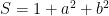 (and
(and  is a certain angle that is now irrelevant at this point in the calculation).
 in terms of
  :
:


![= \displaystyle \frac{ 2 - [ 1 + \tan^2 x])}{1 + \tan^2 x}](https://s0.wp.com/latex.php?latex=%3D+%5Cdisplaystyle+%5Cfrac%7B+2+-+%5B+1+%2B+%5Ctan%5E2+x%5D%29%7D%7B1+%2B+%5Ctan%5E2+x%7D&bg=ffffff&fg=000000&s=0&c=20201002)

 :
: .
. in terms of


 .
. .
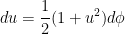
. :
:
![du = \displaystyle \frac{1}{2} \left[ 1 + \tan^2 \displaystyle \frac{\phi}{2} \right] d\phi](https://s0.wp.com/latex.php?latex=du+%3D+%5Cdisplaystyle+%5Cfrac%7B1%7D%7B2%7D+%5Cleft%5B+1+%2B+%5Ctan%5E2+%5Cdisplaystyle+%5Cfrac%7B%5Cphi%7D%7B2%7D+%5Cright%5D+d%5Cphi&bg=ffffff&fg=000000&s=0&c=20201002)