Lagrange Points and Polynomial Equations: Part 4

From Wikipedia, Lagrange points are points of equilibrium for small-mass objects under the gravitational influence of two massive orbiting bodies. There are five such points in the Sun-Earth system, called $L_1$ , $L_2$ , $L_3$ , $L_4$ , and $L_5$ .

The stable equilibrium points $L_4$ and $L_5$ are easiest to explain: they are the corners of equilateral triangles in the plane of Earth’s orbit. The points $L_1$ and $L_2$ are also equilibrium points, but they are unstable. Nevertheless, they have practical applications for spaceflight.

As we’ve seen, the positions of $L_1$ and $L_2$ can be found by numerically solving the fifth-order polynomial equations

$t^5 - (3-\mu) t^4 + (3-2\mu)t^3 - \mu t^2 + 2\mu t - \mu = 0$

and

$t^5 + (3-\mu) t^4 + (3-2\mu)t^3 - \mu t^2 - 2\mu t - \mu = 0$ ,

respectively. In these equations, $\mu = \displaystyle \frac{m_2}{m_1+m_2}$ where $m_1$ is the mass of the Sun and $m_2$ is the mass of Earth. Also, $t$ is the distance from the Earth to $L_1$ or $L_2$ measured as a proportion of the distance from the Sun to Earth.

We’ve also seen that, for the Sun and Earth, $mu \approx 3.00346 \times 10^{-6}$ , and numerically solving the above quintics yields $t \approx 0.000997$ for $L_1$ and $t \approx 0.01004$ for $L_2$ . In other words, $L_1$ and $L_2$ are approximately the same distance from Earth but in opposite directions.

There’s a good reason why the positive real roots of these two similar quintics are almost equal. We know that $t$ will be a lot closer to 0 than 1 because, for gravity to balance, the Lagrange points have to be a lot closer to Earth than the Sun. For this reason, the terms $\mu t^2$ and $2\mu t$ will be a lot smaller than $\mu$ , and so those two terms can be safely ignored in a first-order approximation. Also, the terms $t^5$ and $(3-\mu)t^4$ will be a lot smaller than $(3-2\mu)t^3$ , and so those two terms can also be safely ignored in a first-order approximation. Furthermore, since $\mu$ is also close to 0, the coefficient $(3-2\mu)$ can be safely replaced by just $3$ .

Consequently, the solution of both quintic equations should be close to the solution of the cubic equation

$3t^3 - \mu = 0$ ,

which is straightforward to solve:

$3t^3 = \mu$

$t^3 = \displaystyle \frac{\mu}{3}$

$t = \displaystyle \sqrt[3]{ \frac{\mu}{3} }$ .

If $\mu = 3.00346 \times 10^{-6}$ , we obtain $t \approx 0.010004$ , which is indeed reasonably close to the actual solutions for $L_1$ and $L_2$ . Indeed, this may be used as the first approximation in Newton’s method to quickly numerically evaluate the actual solutions of the two quintic polynomials.

Lagrange Points and Polynomial Equations: Part 3

The position of $L_2$ can be found by numerically solving the fifth-order polynomial equation

$(m_1+m_2)t^5+(3m_1+2m_2)t^4+(3m_1+m_2)t^3$

$-(m_2+3m_3)t^2-(2m_2+3m_3)t-(m_2+m_3)=0$ .

In this equation, $m_1$ is the mass of the Sun, $m_2$ is the mass of Earth, $m_3$ is the mass of the spacecraft, and $t$ is the distance from the Earth to $L_2$ measured as a proportion of the distance from the Sun to Earth. In other words, if the distance from the Sun to Earth is 1 unit, then the distance from the Earth to $L_2$ is $t$ units. The above equation is derived using principles from physics which are not elaborated upon here.

We notice that the coefficients of $t^5$ , $t^4$ , and $t^3$ are all positive, while the coefficients of $t^2$ , $t$ , and the constant term are all negative. Therefore, since there is only one change in sign, this equation has only one positive real root by Descartes’ Rule of Signs.

Since $m_3$ is orders of magnitude smaller than both $m_1$ and $m_2$ , this may safely approximated by

$(m_1+m_2)t^5+(3m_1+2m_2)t^4+(3m_1+m_2)t^3 - m_2 t^2- 2m_2 t-m_2=0$ .

This new equation can be rewritten as

$t^5 + \displaystyle \frac{3m_1 + 2m_2}{m_1 + m_2} t^4 + \frac{3m_1+m_2}{m_1+m_2} t^3 - \frac{m_2}{m_1+m_2} t^2 - \frac{2m_2}{m_1+m_2} t- \frac{m_2}{m_1+m_2} = 0$ .

If we define

$\mu = \displaystyle \frac{m_2}{m_1+m_2}$ ,

we see that

$\displaystyle \frac{3m_1 + 2m_2}{m_1 + m_2} = \frac{3m_1 + 3m_2}{m_1 + m_2} - \frac{m_2}{m_1 + m_2} = 3 - \mu$

and

$\displaystyle \frac{3m_1 + m_2}{m_1 + m_2} = \frac{3m_1 + 3m_2}{m_1 + m_2} - \frac{2m_2}{m_1 + m_2} = 3 - 2\mu$ ,

so that the equation may be written as

$t^5 + (3-\mu) t^4 + (3-2\mu) - \mu t^2 - 2\mu t - \mu = 0$ ,

matching the equation found at Wikipedia.

For the Sun and Earth, $m_1 \approx 1.9885 \times 10^{30} ~ \hbox{kg}$ and $m_2 \approx 5.9724 \times 10^{24} ~ \hbox{kg}$ , so that

$mu = \displaystyle \frac{5.9724 \times 10^{24}}{1.9885 \times 10^{30} + 5.9724 \times 10^{24}} \approx 3.00346 \times 10^{-6}$ .

This yields a quintic equation that is hopeless to solve using standard techniques from Precalculus, but the root can be found graphically by seeing where the function crosses the $x-$ axis (or, in this case, the $t-$ axis):

As it turns out, the root is $t \approx 0.01004$ , so that $L_2$ is located $1.004\%$ of the distance from the Earth to the Sun in the direction away from the Sun.

Lagrange Points and Polynomial Equations: Part 2

We begin with $L_1$ , whose position can be found by numerically solving the fifth-order polynomial equation

$(m_1+m_3)x^5+(3m_1+2m_3)x^4+(3m_1+m_3)x^3$

$-(3m_2+m_3)x^2-(3m_2+m_3)x-(m_2+m_3)=0$ .

In this equation, $m_1$ is the mass of the Sun, $m_2$ is the mass of Earth, $m_3$ is the mass of the spacecraft, and $x$ is the distance from the Earth to $L_1$ measured as a proportion of the distance from the Sun to $L_1$ . In other words, if the distance from the Sun to $L_1$ is 1 unit, then the distance from the Earth to $L_1$ is $x$ units. The above equation is derived using principles from physics which are not elaborated upon here.

We notice that the coefficients of $x^5$ , $x^4$ , and $x^3$ are all positive, while the coefficients of $x^2$ , $x$ , and the constant term are all negative. Therefore, since there is only one change in sign, this equation has only one positive real root by Descartes’ Rule of Signs.

Since $m_3$ is orders of magnitude smaller than both $m_1$ and $m_2$ , this may safely approximated by

$m_1 x^5 + 3m_1 x^4 + 3m_1 x^3 - 3m_2 x^2 - 3m_2x - m_2=0$ .

Unfortunately, the unit $x$ is not as natural for Earth-bound observers as $t$ , the proportion of the distance of $L_1$ to Earth as a proportion of the distance from the Sun to Earth. Since $L_1$ is between the Sun and Earth, the distance from the Sun to Earth is $x+1$ units, so that $t = x/(x+1)$ . We then solve for $x$ in terms of $t$ (just like finding an inverse function):

$t = \displaystyle \frac{x}{x+1}$

$t(x+1) = x$

$tx + t = x$

$t = x - tx$

$t= x(1-t)$

$\displaystyle \frac{t}{1-t} = x$ .

Substituting into the above equation, we find an equation for $t$ :

$\displaystyle \frac{m_1t^5}{(1-t)^5} + \frac{3m_1t^4}{(1-t)^4} + \frac{3m_1t^3}{(1-t)^3} - \frac{3m_2t^2}{(1-t)^2} - \frac{3m_2t}{1-t} - m_2=0$

$m_1t^5 + 3m_1t^4(1-t) + 3m_1t^3(1-t)^2 - 3m_2t^2(1-t)^3 - 3m_2t(1-t)^4 - m_2(1-t)^5=0$

Expanding, we find

$m_1 t^5 + 3m_1 (t^4 - t^5) + 3m_1 (t^3-2t^4+t^5) - 3m_2 (t^2-3t^3+3t^4-t^5)$

$-3m_2(t - 4t^2 + 6t^3 - 4t^4 + t^5) - m_2(1 - 5t + 10t^2 - 10 t^3 + 5t^4 + t^5) = 0$

Collecting like terms, we find

$(m_1 - 3m_1 + 3m_1 + 3m_2 - 3m_2 + m_2)t^5 + (3m_1-6m_1-9m_2+12m_2-5m_2)t^4$

$+ (3m_1+9m_2-18m_2+10m_2)t^3 + (-3m_2+12m_2-10m_2) t^2$

$+ (-3m_2+5m_2)t - m_2 = 0$ ,

$(m_1+m_2) t^5 - (3m_1 +2m_2) t^4 + (3m_1 + m_2) t^3 - m_2 t^2 + 2m_2 t- m_2 = 0$ .

Again, this equation has only one positive real root since the original quintic in $x$ only had one positive real root. This new equation can be rewritten as

$t^5 - \displaystyle \frac{3m_1 + 2m_2}{m_1 + m_2} t^4 + \frac{3m_1+m_2}{m_1+m_2} t^3 - \frac{m_2}{m_1+m_2} t^2 + \frac{2m_2}{m_1+m_2} t- \frac{m_2}{m_1+m_2} = 0$ .

If we define

$\mu = \displaystyle \frac{m_2}{m_1+m_2}$ ,

we see that

$\displaystyle \frac{3m_1 + 2m_2}{m_1 + m_2} = \frac{3m_1 + 3m_2}{m_1 + m_2} - \frac{m_2}{m_1 + m_2} = 3 - \mu$

and

$\displaystyle \frac{3m_1 + m_2}{m_1 + m_2} = \frac{3m_1 + 3m_2}{m_1 + m_2} - \frac{2m_2}{m_1 + m_2} = 3 - 2\mu$ ,

so that the equation may be written as

$t^5 + (\mu-3) t^4 + (3-2\mu) - \mu t^2 + 2\mu t - \mu = 0$ ,

matching the equation found at Wikipedia.

For the Sun and Earth, $m_1 \approx 1.9885 \times 10^{30} ~ \hbox{kg}$ and $m_2 \approx 5.9724 \times 10^{24} ~ \hbox{kg}$ , so that

$\mu = \displaystyle \frac{5.9724 \times 10^{24}}{1.9885 \times 10^{30} + 5.9724 \times 10^{24}} \approx 3.00346 \times 10^{-6}$ .

As it turns out, the root is $t \approx 0.00997$ , so that $L_1$ is located $0.997\%$ of the distance from the Earth to the Sun in the direction of the Sun.

Lagrange Points and Polynomial Equations: Part 1

I recently read a terrific article in the American Mathematical Monthly about Lagrange points, which are (from Wikipedia) “points of equilibrium for small-mass objects under the gravitational influence of two massive orbiting bodies.” There are five such points in the Sun-Earth system, called $L_1$ , $L_2$ , $L_3$ , $L_4$ , and $L_5$ .

To describe these Lagrange points, I can do no better than the estimable Isaac Asimov. I quote from his essay “Colonizing the Heavens” from his book The Beginning and the End, which was published in 1977. I read the book over and over again as a boy in the mid-1980s. (Asimov’s essay originally concerned the Earth-Moon system; in the quote below, I changed the words to apply to the Sun-Earth system.)

Imagine the Sun at zenith, exactly overhead. Trace a line due eastward from the Sun down to the horizon. Two-thirds of the way along that line, one-third of the way up from the horizon, is one of those places. Trace another line westward away from the Sun down to the horizon. Two-thirds of the way along that line, one-third of the way up from the horizon, is another of those places.

Put an object in either place and it will form an equilateral triangle with the Sun and Earth…

What is so special about those places? Back in 1772, the astronomer Joseph Louis Lagrange showed that in those places any object remained stationary with respect to the Sun. As the Earth moved about the Sun, any object in either of those places would also move about the Sun in such a way as to keep perfect step with the Earth. The competing gravities of the Sun and Earth would keep it where it was. If anything happened to push it out of place it would promptly move back, wobbling back and forth a bit (“librating”) as it did so. The two places are called “Lagrangian points” or “libration points.”

Lagrange discovered five such places altogether, but three of them are of no importance since they don’t represent stable conditions. An object in those three places, once pushed out of place, would continue to drift outward and would never return.

The last paragraph of the above quote represents a rare failure of imagination by Asimov, who wrote prolifically about the future of spaceflight. Points $L_4$ and $L_5$ are indeed stable equilibria, and untold science fiction stories have placed spacecraft or colonies at these locations. (The rest of Asimov’s essay speculates about using these points in the Earth-Moon system for space colonization.) However, while the points $L_1$ and $L_2$ are unstable equilibria, they do have practical applications for spacecraft that can perform minor course corrections to stay in position. (The point $L_3$ is especially unstable to outside gravitational influences and thus seems unsuitable for spacecraft.) Again from Wikipedia,

Sun–Earth L₁ is suited for making observations of the Sun–Earth system. Objects here are never shadowed by Earth or the Moon and, if observing Earth, always view the sunlit hemisphere… Solar and heliospheric missions currently located around L₁ include the Solar and Heliospheric Observatory, Wind, Aditya-L1 Mission and the Advanced Composition Explorer. Planned missions include the Interstellar Mapping and Acceleration Probe(IMAP) and the NEO Surveyor.

Sun–Earth L₂ is a good spot for space-based observatories. Because an object around L₂ will maintain the same relative position with respect to the Sun and Earth, shielding and calibration are much simpler… The James Webb Space Telescope was positioned in a halo orbit about L₂ on January 24, 2022.

Earth–Moon L₁ allows comparatively easy access to Lunar and Earth orbits with minimal change in velocity and this has as an advantage to position a habitable space station intended to help transport cargo and personnel to the Moon and back. The SMART-1 Mission passed through the L₁ Lagrangian Point on 11 November 2004 and passed into the area dominated by the Moon’s gravitational influence.

Earth–Moon L₂ has been used for a communications satellite covering the Moon’s far side, for example, Queqiao, launched in 2018, and would be “an ideal location” for a propellant depot as part of the proposed depot-based space transportation architecture.

While the locations $L_4$ and $L_5$ are easy to describe, the precise locations of $L_1$ and $L_2$ are found by numerically solving a fifth-order polynomial equation. This was news to me when I read that article from the American Mathematical Monthly. While I had read years ago that finding the positions of the other three Lagrange points wasn’t simple, I did not realize that it was no more complicated that numerically finding the roots of a polynomial.

The above article from the American Mathematical Monthly concludes…

[t]he mathematical tools that Lagrange uses to arrive at a solution to this three-body problem lie entirely within the scope of modern courses in algebra, trigonometry, and first-semester calculus. But surely no ordinary person could have pursued the many extraordinarily complicated threads in his work to their ends, let alone woven them together into a magnificent solution to the problem as he has done. Lagrange noted in the introduction to his essay, “This research is really no more than for pure curiosity …” If only he could have watched on Christmas Day as the James Webb Space Telescope began its journey to the Lagrange point $L_2$ !

In this short series, we discuss the polynomial equations for finding $L_1$ and $L_2$ .

Predicate Logic and Popular Culture: Index

I’m doing something that I should have done a long time ago: collecting a series of posts into one single post. The following links comprised my series on using examples from popular culture to illustrate principles of predicate logic. My experiences teaching these ideas to my discrete mathematics students led to my recent publication (John Quintanilla, “Name That Tune: Teaching Predicate Logic with Popular Culture,” MAA Focus, Vol. 36, No. 4, pp. 27-28, August/September 2016).

Unlike other series that I’ve made, this series didn’t have a natural chronological order. So I’ll list these by concept illustrated from popular logic. The vast majority of these examples were suggested by my students.

Logical and $\land$ :

Part 1: “You Belong To Me,” by Taylor Swift
Part 21: “Do You Hear What I Hear,” covered by Whitney Houston
Part 31: The Godfather (1972)
Part 45: The Blues Brothers (1980)
Part 53: “What Does The Fox Say,” by Ylvis
Part 54: “Billie Jean,” by Michael Jackson
Part 98: “Call Me Maybe,” by Carly Rae Jepsen.
Part 137: “Pen Pineapple Apple Pen,” by Pikotaro.
Part 142: “Galway Girl,” by Ed Sheeran.
Part 183: A memorable line from Avengers: Age of Ultron.
Part 184: A memorable line from Star Wars Episode I: The Phantom Menace.
Part 197: “That’s Life,” by Frank Sinatra.
Part 209: A line from The Office.
Part 242: A line from The Fellowship of the Ring.
Part 249: “We Didn’t Start the Fire,” by Billy Joel.
Part 252: A line from The Two Towers.
Part 253: “I’m Gonna Miss Her,” by Brad Paisley.
Part 261: A line from Spiderman 2.

Logical or $\lor$ :

Part 1: Shawshank Redemption (1994)

Logical negation $\lnot$ :

Part 1: Richard Nixon
Part 32: “Satisfaction!”, by the Rolling Stones
Part 39: “We Are Never Ever Getting Back Together,” by Taylor Swift
Part 129: “Blue Ain’t Your Color,” by Keith Urban.
Part 143: “Ain’t Worth The Whiskey,” by Cole Swindell.
Part 247: A line from The Fellowship of the Ring.

Logical implication $\Rightarrow$ :

Part 1: Field of Dreams (1989), and also “Roam,” by the B-52s
Part 2: “Word Crimes,” by Weird Al Yankovic
Part 7: “I’ll Be There For You,” by The Rembrandts (Theme Song from Friends)
Part 43: “Kiss,” by Prince
Part 50: “I’m Still A Guy,” by Brad Paisley
Part 76: “You’re Never Fully Dressed Without A Smile,” from Annie.
Part 109: “Dancing in the Dark,” by Bruce Springsteen.
Part 122: “Keep Yourself Alive,” by Queen.
Part 140: “It Don’t Mean A Thing If It Ain’t Got That Swing,” by Ella Fitzgerald.
Part 174: A famous line from Rocky IV.
Part 176: A famous line from Game of Thrones.
Part 185: A line from Westworld.
Part 188: A line from Talladega Nights.
Part 195: “If We Were a Movie,” from the Hannah Montana series.
Part 207: A line from Name of the Wind, by Patrick Rothfuss.
Part 222: A line from The Notebook.
Part 234: “Battle Symphony,” by Linkin Park.
Part 235: A line from Suits.
Part 259: “Out There,” from “The Hunchback of Notre Dame.”
Part 269: “Dear Theodosia,” from Hamilton.

For all $\forall$ :

Part 3: Casablanca (1942)
Part 4: A Streetcar Named Desire (1951)
Part 34: “California Girls,” by The Beach Boys
Part 37: Fellowship of the Ring, by J. R. R. Tolkien
Part 49: “Buy Me A Boat,” by Chris Janson
Part 57: “Let It Go,” by Idina Menzel and from Frozen (2013)
Part 65: “Stars and Stripes Forever,” by John Philip Sousa.
Part 68: “Love Yourself,” by Justin Bieber.
Part 69: “I Will Always Love You,” by Dolly Parton (covered by Whitney Houston).
Part 74: “Faithfully,” by Journey.
Part 79: “We’re Not Gonna Take It Anymore,” by Twisted Sister.
Part 87: “Hungry Heart,” by Bruce Springsteen.
Part 99: “It’s the End of the World,” by R.E.M.
Part 100: “Hold the Line,” by Toto.
Part 101: “Break My Stride,” by Matthew Wilder.
Part 102: “Try Everything,” by Shakira.
Part 108: “BO$$,” by Fifth Harmony.
Part 113: “Sweet Caroline,” by Neil Diamond.
Part 114: “You Know Nothing, Jon Snow,” from Game of Thrones.
Part 118: “The Lazy Song,” by Bruno Mars.
Part 120: “Cold,” by Crossfade.
Part 123: “Always on My Mind,” by Willie Nelson.
Part 127: Motif from Hamilton.
Part 131: Abraham Lincoln’s Second Inaugural Address.
Part 132: A famous line from The Fellowship of the Ring.
Part 133: A famous line from Braveheart.
Part 136: “I Don’t Wanna Live Forever,” by ZAYN and Taylor Swift.
Part 138: “Bohemian Rhapsody,” by Queen.
Part 144: “The Anchor,” by Bastille.
Part 146: A line from the video game series “Fallout”
Part 147: “Nobody’s Perfect,” from the Hannah Montana series.
Part 150: “Roar,” by Katy Perry.
Part 167: “Look What You Made Me Do,” by Taylor Swift.
Part 180: “Bohemian Rhapsody,” by Queen.
Part 181: “We Don’t Talk Anymore,” by Charlie Puth and Selena Gomez.
Part 189: “Tengo Muchas Alas / I Have Many Wings,” by Mana.
Part 190: “Eastside,” by Benny Blanco, Halsey, and Khalid.
Part 191: “I’m a Mess,” by Bebe Rexha.
Part 193: “Forever and Ever, Amen,” by Randy Travis.
Part 202: “Everything Is Awesome!!!,” from The Lego Movie.
Part 204: “She’s Always A Woman,” by Billy Joel.
Part 208: A line by Naruto in Masashi Kishimoto’s anime.
Part 211: “Everyone Lies To Me,” by Knuckle Puck.
Part 214: “Aeroplane,” by Björk.
Part 216: “Hound Dog,” by Elvis Presley.
Part 227: One Fish, Two Fish, Red Fish, Blue Fish, by Dr. Seuss.
Part 230: “Be Alright,” by Dean Lewis.
Part 231: “Everyone Wants To Be A Cat,” from The Aristocats.
Part 232: “Behind Blue Eyes,” by Limp Bizkit.
Part 236: A line from Dirty Dancing.
Part 243: “Better,” by Khalid.
Part 246: “Unfaithful,” by Rihanna.
Part 260: A line from Ratatouille.
Part 263: A line from Shakespeare’s As You Like It.
Part 264: “Bet On It,” from High School Musical 2.
Part 271: A line from Pirates of the Caribbean: The Curse of the Black Pearl.
Part 273: “Gaston,” from Beauty and the Beast.

For all and implication:

Part 8 and Part 9: “What Makes You Beautiful,” by One Direction
Part 13: “Safety Dance,” by Men Without Hats
Part 16: The Fellowship of the Ring, by J. R. R. Tolkien
Part 24 : “The Chipmunk Song,” by The Chipmunks
Part 55: The Quiet Man (1952)
Part 62: “All My Exes Live In Texas,” by George Strait.
Part 70: “Wannabe,” by the Spice Girls.
Part 72: “You Shook Me All Night Long,” by AC/DC.
Part 81: “Ascot Gavotte,” from My Fair Lady
Part 82: “Sharp Dressed Man,” by ZZ Top.
Part 86: “I Could Have Danced All Night,” from My Fair Lady.
Part 95: “Every Breath You Take,” by The Police.
Part 96: “Only the Lonely,” by Roy Orbison.
Part 97: “I Still Haven’t Found What I’m Looking For,” by U2.
Part 105: “Every Rose Has Its Thorn,” by Poison.
Part 107: “Party in the U.S.A.,” by Miley Cyrus.
Part 112: “Winners Aren’t Losers,” by Donald J. Trump and Jimmy Kimmel.
Part 115: “Every Time We Touch,” by Cascada.
Part 117: “Stronger,” by Kelly Clarkson.
Part 125: “Do Wot You Do,” by INXS.
Part 130: “Think of You,” by Chris Young and Cassadee Pope.
Part 135: “Can’t Feel My Face,” by The Weeknd.
Part 145: A line from Black Dynamite.
Part 152: “You Haven’t Done Nothin’,” by Stevie Wonder.
Part 155: “All The Lazy Boyfriends,” by They Might Be Giants.
Part 165: A famous quote by Eleanor Roosevelt.
Part 166: “Perfect,” by Ed Sheeran.
Part 172: “Twas the Night Before Christmas,” by Clement Clarke Moore.
Part 182: “How Far I’ll Go,” from Moana.
Part 192: A line from the videogame “Overwatch.”
Part 194: A line from the Dragon Ball franchise.
Part 196: “ME!,” by Taylor Swift.
Part 200: A line from the 1990s Spider-Man cartoons.
Part 201: “It’s Quiet Uptown,” from Hamilton.
Part 205: “Three Little Birds,” by Bob Marley.
Part 206: “Mudfootball,” by Jack Johnson.
Part 210: “On My Way,” by Alan Walker, Sabrina Carpenter, and Farruko.
Part 215: “Aging Rockers,” by Tim Hawkins.
Part 218: “Happy Together,” by The Turtles.
Part 223: “Too Deep to Turn Back,” by Daniel Caesar.
Part 224: “Nothing Gold Can Stay,” by Robert Frost.
Part 225: “He Stopped Loving Her Today,” by George Jones.
Part 229: A line from Mean Girls.
Part 233: “Emperor’s New Clothes,” by Panic! At The Disco.
Part 240: “For Those About To Rock (We Salute You),” by AC/DC.
Part 244: A famous line from Spiderman.
Part 248: The poem “All That Is Gold Does Not Glitter,” from The Fellowship of the Ring.
Part 251: “Survey Ladies,” from Animaniacs.
Part 265: “Every Time You Go Away,” by Paul Young.
Part 268: “Sweet Dreams,” by Eurhymics.
Part 270: A line from the anime “Naruto Shippuden.”
Part 272: “Be Our Guest,” from Beauty and the Beast.
Part 274: “He Stopped Loving Her Today,” by George Jones.

There exists $\exists$ :

Part 10: “Unanswered Prayers,” by Garth Brooks
Part 15: “Stand by Your Man,” by Tammy Wynette (also from The Blues Brothers)
Part 36: Hamlet, by William Shakespeare
Part 57: “Let It Go,” by Idina Menzel and from Frozen (2013)
Part 93: “There’s No Business Like Show Business,” from Annie Get Your Gun (1946).
Part 94: “Not While I’m Around,” from Sweeney Todd (1979).
Part 104: “Wild Blue Yonder” (US Air Force)
Part 106: “No One,” by Alicia Keys.
Part 116: “Ocean Front Property,” by George Strait.
Part 139: “Someone in the Crowd,” from La La Land.
Part 149: “Someone Like You,” by Adele.
Part 151: “E-MO-TION,” by Carly Rae Jepsen.
Part 154: “I Wanna Dance With Somebody,” by Whitney Houston.
Part 162: “Think of You,” by Chris Young and Cassadee Pope.
Part 168: “Sorry,” by Halsey.
Part 175: “Someday We’ll Be Together,” by Diana Ross and the Supremes.
Part 177: “Try Everything,” by Shakira.
Part 186: “Someday,” by Nickelback.
Part 226: “The Wizard and I,” from Wicked.
Part 238: A line from the video game “Among Us.”
Part 250: “Ain’t No Mountain High Enough,” by Marvin Gaye.

Existence and uniqueness:

Part 14: “Girls Just Want To Have Fun,” by Cyndi Lauper
Part 20: “All I Want for Christmas Is You,” by Mariah Carey
Part 23: “All I Want for Christmas Is My Two Front Teeth,” covered by The Chipmunks
Part 29: “You’re The One That I Want,” from Grease
Part 30: “Only You,” by The Platters
Part 35: “Hound Dog,” by Elvis Presley
Part 73: “Dust In The Wind,” by Kansas.
Part 75: “Happy Together,” by The Turtles.
Part 77: “All She Wants To Do Is Dance,” by Don Henley.
Part 90: “All You Need Is Love,” by The Beatles.
Part 169: “Marry Me,” by Thomas Rhett.
Part 179: A line from “Harry Potter and the Sorcerer’s Stone.”
Part 245: An advertising line for Gibson guitars.
Part 258: “Nobody Knows,” by Kevin Sharp.
Part 262: “Dust in the Wind,” by Kansas.

DeMorgan’s Laws:

Part 5: “Never Gonna Give You Up,” by Rick Astley
Part 28: “We’re Breaking Free,” from High School Musical (2006)
Part 255: A line from “The Nightmare Before Christmas.”
Part 257: A line from “The Wizard of Oz.”

Simple nested predicates:

Part 6: “Everybody Loves Somebody Sometime,” by Dean Martin
Part 25: “Every Valley Shall Be Exalted,” from Handel’s Messiah
Part 33: “Heartache Tonight,” by The Eagles
Part 38: “Everybody Needs Somebody To Love,” by Wilson Pickett and covered in The Blues Brothers (1980)
Part 46: “Mean,” by Taylor Swift
Part 56: “Turn! Turn! Turn!” by The Byrds
Part 63: P. T. Barnum.
Part 64: Abraham Lincoln.
Part 66: “Somewhere,” from West Side Story.
Part 71: “Hold On,” by Wilson Philips.
Part 80: Liverpool FC.
Part 84: “If You Leave,” by OMD.
Part 103: “The Caisson Song” (US Army).
Part 111: “Always Something There To Remind Me,” by Naked Eyes.
Part 121: “All the Right Moves,” by OneRepublic.
Part 126: Motif from Hamilton.
Part 157: “Whenever, Wherever,” by Shakira.
Part 158: “Church Bells,” by Carrie Underwood.
Part 163: A famous line from The Princess Bride.
Part 170: “Everywhere,” by Tim McGraw.
Part 173: “If I Ain’t Got You,” by Alicia Keys.
Part 187: “Always Something There To Remind Me,” by Naked Eyes.
Part 198: “All Star,” by Smash Mouth.
Part 203: “Lean On Me,” by Bill Withers.
Part 217: A line in the video game Valorant.
Part 219: “Señorita,” by Shawn Mendes and Camila Cabello.
Part 220: “How to Love,” by Cash Cash.
Part 221: A line from Monk.
Part 237: A line from Psycho.
Part 254: “You Can’t Always Get What You Want,” by the Rolling Stones.
Part 256: “Irgendwie, Irgendwo, Irgendwann” by Nena.
Part 266: “Kokomo,” by the Beach Boys.

Maximum or minimum of a function:

Part 12: “For the First Time in Forever,” by Kristen Bell and Idina Menzel and from Frozen (2013)
Part 19: “Tennessee Christmas,” by Amy Grant
Part 22: “The Most Wonderful Time of the Year,” by Andy Williams
Part 48: “I Got The Boy,” by Jana Kramer
Part 60: “I Loved Her First,” by Heartland
Part 92: “Anything You Can Do,” from Annie Get Your Gun.
Part 119: “Uptown Girl,” by Billy Joel.
Part 124: “All I Want To Do Is Be With You,” from High School Musical 3.
Part 160: “God, Your Mama, and Me,” by Florida Georgia Line and the Backstreet Boys.
Part 178: “Ex Factor,” by Lauryn Hill.

Somewhat complicated examples:

Part 11 : “Friends in Low Places,” by Garth Brooks
Part 27 : “There is a Castle on a Cloud,” from Les Miserables
Part 41: Winston Churchill
Part 44: Casablanca (1942)
Part 51: “Everybody Wants to Rule the World,” by Tears For Fears
Part 58: “Fifteen,” by Taylor Swift
Part 59: “We Are Never Ever Getting Back Together,” by Taylor Swift
Part 61: “Style,” by Taylor Swift
Part 67: “When I Think Of You,” by Janet Jackson.
Part 78: “Nothing’s Gonna Stop Us Now,” by Starship.
Part 89: “No One Is Alone,” from Into The Woods.
Part 110: “Everybody Loves My Baby,” by Louis Armstrong.
Part 134: A famous line from Braveheart.
Part 141: “How Far I’ll Go,” from Moana.
Part 148: “The Climb,” by Miley Cyrus.
Part 153: “I Can’t Tell You Why,” by The Eagles.
Part 161: “For What It’s Worth,” by Buffalo Springfield.
Part 164: “When The Sun Goes Down,” by Kenny Chesney.
Part 199: “Never Say Never,” by Justin Bieber.
Part 213: “Sign of the Times,” by Harry Styles.
Part 241: “Dreams,” by Fleetwood Mac.
Part 267: A line from The Hound of the Baskervilles.

Fairly complicated examples:

Part 17 : Richard Nixon
Part 47: “Homegrown,” by Zac Brown Band
Part 52: “If Ever You’re In My Arms Again,” by Peabo Bryson
Part 83: “Something Good,” from The Sound of Music.
Part 85: “Joy To The World,” by Three Dog Night.
Part 88: “Like A Rolling Stone,” by Bob Dylan.
Part 91: “Into the Fire,” from The Scarlet Pimpernel.
Part 128: “A Puzzlement,” from The King and I.
Part 156: “Everybody Loves a Lover,” by Doris Day.
Part 159: “Fastest Girl in Town,” by Miranda Lambert.
Part 171: “Everybody’s Got Somebody But Me,” by Hunter Hayes.

Really complicated examples:

Part 18: “Sleigh Ride,” covered by Pentatonix
Part 26: “All the Gold in California,” by the Gatlin Brothers
Part 40: “One of These Things Is Not Like the Others,” from Sesame Street
Part 42: “Take It Easy,” by The Eagles

Mathematical Allusions in Shantaram (Part 1)

I recently finished the novel Shantaram, by Gregory David Roberts. As I’m not a professional book reviewer, let me instead quote from the Amazon review:

Crime and punishment, passion and loyalty, betrayal and redemption are only a few of the ingredients in Shantaram, a massive, over-the-top, mostly autobiographical novel. Shantaram is the name given Mr. Lindsay, or Linbaba, the larger-than-life hero. It means “man of God’s peace,” which is what the Indian people know of Lin. What they do not know is that prior to his arrival in Bombay he escaped from an Australian prison where he had begun serving a 19-year sentence. He served two years and leaped over the wall. He was imprisoned for a string of armed robberies performed to support his heroin addiction, which started when his marriage fell apart and he lost custody of his daughter. All of that is enough for several lifetimes, but for Greg Roberts, that’s only the beginning.

He arrives in Bombay with little money, an assumed name, false papers, an untellable past, and no plans for the future. Fortunately, he meets Prabaker right away, a sweet, smiling man who is a street guide. He takes to Lin immediately, eventually introducing him to his home village, where they end up living for six months. When they return to Bombay, they take up residence in a sprawling illegal slum of 25,000 people and Linbaba becomes the resident “doctor.” With a prison knowledge of first aid and whatever medicines he can cadge from doing trades with the local Mafia, he sets up a practice and is regarded as heaven-sent by these poor people who have nothing but illness, rat bites, dysentery, and anemia. He also meets Karla, an enigmatic Swiss-American woman, with whom he falls in love. Theirs is a complicated relationship, and Karla’s connections are murky from the outset.

While it was a cracking good read, what struck me particularly were the surprising mathematical allusions that the author used throughout the novel. In this mini-series, I’d like to explore the ones that I found.

In this first installment, the narrator describes a life-or-death situation as he is being choked:

He was a hard man. He didn’t give up. His hands squeezed tighter. My neck was strong and the muscles were well developed, but I knew he had the strength to kill me. My hand reached, groping for the pistol in my pocket. I had to shoot him. I had to kill him. That was all right. I didn’t care. The air in my lungs was spent, and my brain was exploding in Mandelbrot whirls of colored light, and I was dying, and I wanted to kill him.
Shantaram, Chapter 25

Someone being choked to death might be prosaically described as “seeing stars,” but the author instead to choose the more vivid imagery of “exploding in Mandelbrot whirls of colored light.” The Mandelbrot set is a fractal that solves a famous mathematical problem:

And the Mandelbrot set is quite colorful and complex, which might indeed be a better description than “seeing stars” of what might be going through someone’s mind when being choked to death. Although somewhat dated, here’s my favorite Mandelbrot zoom video:

Confirming Einstein’s Theory of General Relativity With Calculus, Part 8: Second- and Third-Order Approximations

In this series, I’m discussing how ideas from calculus and precalculus (with a touch of differential equations) can predict the precession in Mercury’s orbit and thus confirm Einstein’s theory of general relativity. The origins of this series came from a class project that I assigned to my Differential Equations students maybe 20 years ago.

In this series, we found an approximate solution to the governing initial-value problem

$u''(\theta) + u(\theta) = \displaystyle \frac{1}{\alpha} + \delta [u(\theta)]^2$

$u(0) = \displaystyle \frac{1 + \epsilon}{\alpha}$

$u'(0) = 0$ ,

where $u = \displaystyle \frac{1}{r}$ , $\displaystyle \frac{1}{\alpha} = \frac{GMm^2}{\ell^2}$ , $\delta = \displaystyle \frac{3GM}{c^2}$ , $G$ is the gravitational constant of the universe, $m$ is the mass of the planet, $M$ is the mass of the Sun, $\ell$ is the constant angular momentum of the planet, $\epsilon$ is the eccentricity of the orbit, and $c$ is the speed of light.

We used the following steps to find an approximate solution.

Step 0. Ignore the general-relativity contribution and solve the simpler initial-value problem

$u_0''(\theta) + u_0(\theta) = \displaystyle \frac{1}{\alpha}$

$u_0(0) = \displaystyle \frac{1 + \epsilon}{\alpha}$

$u_0'(0) = 0$ ,

which is a zeroth-order approximation to the real initial-value problem. We found that the solution of this differential equation is

$u_0(\theta) = \displaystyle \frac{1 + \epsilon \cos \theta}{\alpha}$ ,

which is the equation of an ellipse in polar coordinates.

Step 1. Solve the initial-value problem

$u_1''(\theta) + u_1(\theta) = \displaystyle \frac{1}{\alpha} + \delta [u_0(\theta)]^2$

$u_1(0) = \displaystyle \frac{1 + \epsilon}{\alpha}$

$u_1'(0) = 0$ ,

which partially incorporates the term due to general relativity. This is a first-order approximation to the real differential equation. After much effort, we found that the solution of this initial-value problem is

$u_1(\theta) = \displaystyle \frac{1 + \epsilon \cos \theta}{\alpha} + \frac{\delta}{\alpha^2} + \frac{\delta \epsilon^2}{2\alpha^2} + \frac{ \delta\epsilon}{\alpha^2} \theta \sin \theta - \frac{ \delta \epsilon^2}{6\alpha^2} \cos 2\theta - \frac{\delta(3+\epsilon^2)}{3\alpha^2} \cos \theta$ .

For large values of $\theta$ , this is accurately approximated as:

$u_1(\theta) \approx \displaystyle \frac{1 + \epsilon \cos \theta}{\alpha} + \frac{ \delta\epsilon}{\alpha^2} \theta \sin \theta$ ,

which can be further approximated as

$u_1(\theta) \approx \displaystyle \frac{1}{\alpha} \left[ 1 + \epsilon \cos \left( \theta - \frac{\delta \theta}{\alpha} \right) \right]$ .

From this expression, the precession in a planet’s orbit due to general relativity can be calculated.

Roughly 20 years ago, I presented this application of differential equations at the annual meeting of the Texas Section of the Mathematical Association of America. After the talk, a member of the audience asked what would happen if we did this procedure yet again to find a second-order approximation. In other words, I was asked to consider…

Step 2. Solve the initial-value problem

$u_2''(\theta) + u_2(\theta) = \displaystyle \frac{1}{\alpha} + \delta [u_1(\theta)]^2$

$u_2(0) = \displaystyle \frac{1 + \epsilon}{\alpha}$

$u_2'(0) = 0$ .

It stands to reason that the answer should be an even more accurate approximation to the true solution $u(\theta)$ .

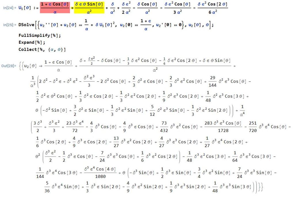
I didn’t have an immediate answer for this question, but I can answer it now. Letting Mathematica do the work, here’s the answer:

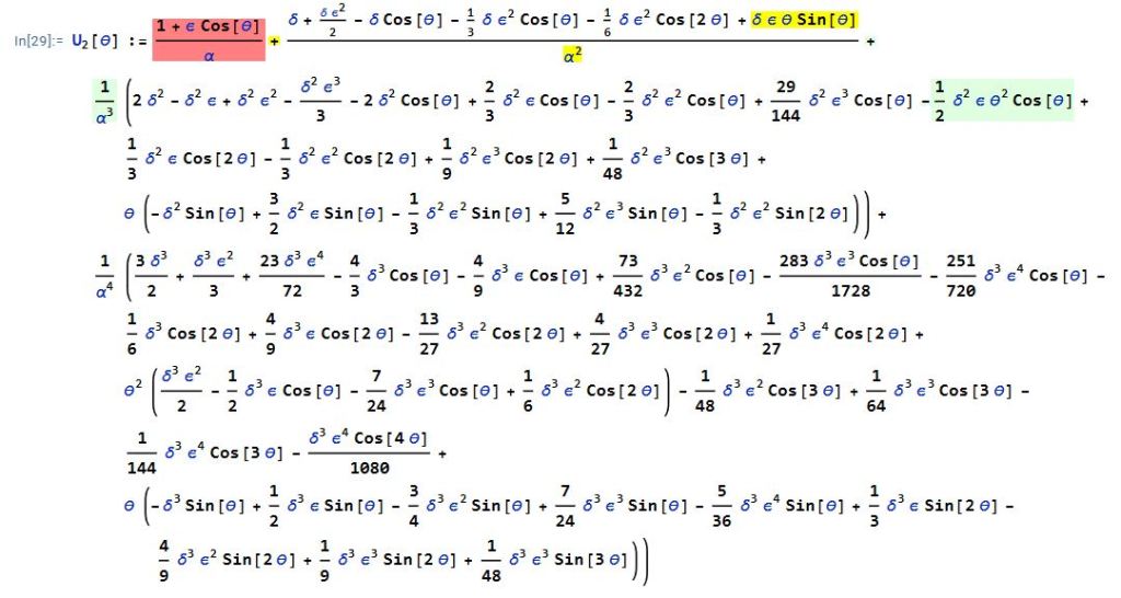
Yes, it’s a mess. The term in red is $u_0(\theta)$ , while the term in yellow is the next largest term in $u_1(\theta)$ . Both of these appear in the answer to $u_2(\theta)$ .

The term in green is the next largest term in $u_2(\theta)$ , with the highest power of $\theta$ in the numerator and the highest power of $\alpha$ in the denominator. In other words,

$u_2(\theta) \approx \displaystyle \frac{1 + \epsilon \cos \theta}{\alpha} + \frac{ \delta\epsilon}{\alpha^2} \theta \sin \theta -\frac{\delta^2 \epsilon}{2\alpha^3} \theta^2 \cos \theta$ .

How does this compare to our previous approximation of

$u(\theta) \approx \displaystyle \frac{1}{\alpha} \left[ 1 + \epsilon \cos \left( \theta - \frac{\delta \theta}{\alpha} \right) \right]$ ?

Well, to a second-order Taylor approximation, it’s the same! Let

$f(x) = \displaystyle \frac{1}{\alpha} \left[ 1 + \epsilon \cos \left( \theta - x \right) \right]$ .

Expanding about $x = 0$ and treated $\theta$ as a constant, we find

$f(x) \approx f(0) + f'(0) x + \displaystyle \frac{f''(0)}{2} x^2 = \displaystyle \frac{1}{\alpha} \left[ 1 + \epsilon \cos \left( \theta\right) \right] + \frac{\epsilon}{\alpha} x \sin \theta - \frac{\epsilon}{2\alpha} x^2 \cos \theta$ .

Substituting $x = \displaystyle \frac{\delta \theta}{\alpha}$ yields the above approximation for $u_2(\theta)$ .

Said another way, proceeding to a second-order approximation merely provides additional confirmation for the precession of a planet’s orbit.

Just for the fun of it, I also used Mathematica to find the solution of Step 3:

Step 2. Solve the initial-value problem

$u_3''(\theta) + u_3(\theta) = \displaystyle \frac{1}{\alpha} + \delta [u_2(\theta)]^2$

$u_3(0) = \displaystyle \frac{1 + \epsilon}{\alpha}$

$u_3'(0) = 0$ .

I won’t copy-and-paste the solution from Mathematica; unsurpisingly, it’s really long. I will say that, unsurprisingly, the leading terms are

$u_3(\theta) \approx \displaystyle \frac{1 + \epsilon \cos \theta}{\alpha} + \frac{ \delta\epsilon}{\alpha^2} \theta \sin \theta -\frac{\delta^2 \epsilon}{2 \alpha^3} \theta^2 \cos \theta -\frac{\delta^3 \epsilon}{6\alpha^4} \theta^3 \sin \theta$ .

I said “unsurprisingly” because this matches the third-order Taylor polynomial of our precession expression. I don’t have time to attempt it, but surely there’s a theorem to be proven here based on this computational evidence.

Confirming Einstein’s Theory of General Relativity With Calculus, Part 7e: Computing Precession

We have shown that under general relativity, the motion of a planet around the Sun precesses by

$\phi = \displaystyle \frac{6\pi GM}{ac^2 (1-\epsilon^2)} \qquad \hbox{radians per orbit}$ ,

where $a$ is the semi-major axis of the planet’s orbit, $\epsilon$ is the orbit’s eccentricity, $G$ is the gravitational constant of the universe, $M$ is the mass of the Sun, and $c$ is the speed of light.

Notice that for $\phi$ to be as observable as possible, we’d like $a$ to be as small as possible and $\epsilon$ to be as large as possible. By a fortunate coincidence, the orbit of Mercury — the closest planet to the sun — has the most elliptical orbit of the eight planets.

Here are the values of the constants for Mercury’s orbit in the SI system:

$G = 6.6726 \times 10^{-11} \qquad \hbox{N-m}^2/\hbox{kg}^2$
$M = 1.9929 \times 10^{30} \qquad \hbox{kg}$
$a = 5.7871 \times 10^{10} \qquad \hbox{m}$
$c = 2.9979 \times 10^{8} \qquad \hbox{m/s}$
$\epsilon = 0.2056$
$T = 0.2408 \qquad \hbox{years}$

The last constant, $T$ , is the time for Mercury to complete one orbit. This isn’t in the SI system, but using Earth years as the unit of time will prove useful later in this calculation.

Using these numbers, and recalling that $1 ~ \hbox{N} = 1 ~ \hbox{kg-m/s}^2$ , we find that

$\phi = \displaystyle \frac{6\pi \times 6.6726 \times 10^{-11} ~ \hbox{m}^3/(\hbox{kg-s}^2) \times 1.9929 \times 10^{30} ~ \hbox{kg}}{5.7871 \times 10^{10} ~ \hbox{m} \times (2.9979 \times 10^{8} ~ \hbox{m/s})^2 \times (1-(0.2408)^2)} \approx 5.03 \times 10^{-7}$ .

Notice that all of the units cancel out perfectly; this bit of dimensional analysis is a useful check against careless mistakes.

Again, the units of $\phi$ are in radians per Mercury orbit, or radians per 0.2408 years. We now convert this to arc seconds per century:

$\phi \approx 5.03 \times 10^{-7} \displaystyle \frac{\hbox{radians}}{\hbox{0.2408 years}} \times \frac{180 ~\hbox{degrees}}{\pi ~ \hbox{radians}} \times \frac{3600 ~ \hbox{arc seconds}}{1 ~ \hbox{degree}} \times \frac{100 ~ \hbox{years}}{1 ~ \hbox{century}}$

$\phi = 43.1 \displaystyle \frac{\hbox{arc seconds}}{\hbox{century}}$ .

This indeed matches the observed precession in Mercury’s orbit, thus confirming Einstein’s theory of relativity.

This same computation can be made for other planets. For Venus, we have the new values of $a = 1.0813 \times 10^{11} ~ \hbox{m}$ , $\epsilon = 0.0068$ , and $T = 0.6152 ~ \hbox{years}$ . Repeating this calculation, we predict the precession in Venus’s orbit to be 8.65” per century. Einstein made this prediction in 1915, when the telescopes of the time were not good enough to measure the precession in Venus’s orbit. This only happened in 1960, 45 years later and 5 years after Einstein died. Not surprisingly, the precession in Venus’s orbit also agrees with general relativity.

Confirming Einstein’s Theory of General Relativity With Calculus, Part 7d: Predicting Precession IV

We have shown that the motion of a planet around the Sun, expressed in polar coordinates $(r,theta)$ with the Sun at the origin, under general relativity is

$u(\theta) \approx \displaystyle \frac{1}{\alpha} \left[ 1 + \epsilon \cos \left( \theta - \frac{\delta \theta}{\alpha} \right) \right]$ ,

where $u = \displaystyle \frac{1}{r}$ , $\alpha = a(1-\epsilon^2)$ , $a$ is the semi-major axis of the planet’s orbit, $\epsilon$ is the orbit’s eccentricity, $\delta = \displaystyle \frac{3GM}{c^2}$ , $G$ is the gravitational constant of the universe, $m$ is the mass of the planet, $M$ is the mass of the Sun, $P$ is the planet’s perihelion, $\ell$ is the constant angular momentum of the planet, and $c$ is the speed of light.

The above function $u(\theta)$ is maximized (i.e., the distance from the Sun $r(\theta)$ is minimized) when $\displaystyle \cos \left( \theta - \frac{\delta \theta}{\alpha} \right)$ is as large as possible. This occurs when $\theta - \displaystyle \frac{\delta \theta}{\alpha}$ is a multiple of $2\pi$ .

Said another way, the planet is at its closest point to the Sun when $\theta = 0$ . One orbit later, the planet returns to its closest point to the Sun when

$\theta - \displaystyle \frac{\delta \theta}{\alpha} = 2\pi$

$\theta \displaystyle\left(1 - \frac{\delta}{\alpha} \right) = 2\pi$

$\theta = 2\pi \displaystyle\frac{1}{1 - (\delta/\alpha)}$

We now use the approximation

$\displaystyle \frac{1}{1-x} \approx 1 + x \qquad \hbox{if} \qquad x \approx 0$ ;

this can be demonstrated by linearization, Taylor series, or using the first two terms of the geometric series $1 + x + x^2 + x^3 + \dots$ . With this approximation, the closest approach to the Sun in the next orbit occurs when

$\theta = 2\pi \displaystyle\left(1 + \frac{\delta}{\alpha} \right) = 2\pi + \frac{2\pi \delta}{\alpha}$ ,

which is coterminal with the angle

$\phi = \displaystyle \frac{2\pi \delta}{\alpha}$ .

Substituting $\alpha = a(1-\epsilon^2)$ and $\delta = \displaystyle \frac{3GM}{c^2}$ , we see that the amount of precession per orbit is

$\phi = \displaystyle 2 \pi \frac{3GM}{c^2} \frac{1}{a(1-\epsilon^2)} = \frac{6\pi G M}{ac^2(1-\epsilon^2)}$ .

The units of $\phi$ are radians per orbit. In the next post, we will use Mercury’s data to find $\phi$ in seconds of arc per century.

Confirming Einstein’s Theory of General Relativity With Calculus, Part 7c: Predicting Precession III

We have shown that the motion of a planet around the Sun, expressed in polar coordinates $(r,theta)$ with the Sun at the origin, under general relativity is

$u(\theta) \approx \displaystyle \frac{1}{\alpha} \left[ 1 + \epsilon \cos \left( \theta - \frac{\delta \theta}{\alpha} \right) \right]$ ,

where $u = \displaystyle \frac{1}{r}$ , $\displaystyle \frac{1}{\alpha} = \frac{GMm^2}{\ell^2}$ , $\epsilon = \displaystyle \frac{\alpha - P}{P}$ , $\delta = \displaystyle \frac{3GM}{c^2}$ , $G$ is the gravitational constant of the universe, $m$ is the mass of the planet, $M$ is the mass of the Sun, $P$ is the planet’s perihelion, $\ell$ is the constant angular momentum of the planet, and $c$ is the speed of light.

We notice that the orbit of a planet under general relativity looks very, very similar to the orbit under Newtonian physics:

$u(\theta) \approx \displaystyle \frac{1}{\alpha} \left[ 1 + \epsilon \cos \theta \right]$ ,

so that

$r(\theta) = \displaystyle \frac{\alpha}{1 + \epsilon \cos \theta}$ .

As we’ve seen, this describes an elliptical orbit, normally expressed in rectangular coordinates as

$\displaystyle \frac{(x-h)^2}{a^2} + \frac{y^2}{b^2} = 1$ ,

with semimajor axis along the $x-$ axis. In particular, for an elliptical orbit, the planet’s closest approach to the Sun occurs at $\theta = 0$ :

$r(0) = \displaystyle \frac{\alpha}{1 + \epsilon \cos 0} = \frac{\alpha}{1 + \epsilon}$ ,

and the planet’s further distance from the Sun occurs at $\theta = \pi$ :

$r(\pi) = \displaystyle \frac{\alpha}{1 + \epsilon \cos \pi} = \frac{\alpha}{1 - \epsilon}$ .

Therefore, the length $2a$ of the major axis of the ellipse is the sum of these two distances:

$2a = \displaystyle \frac{\alpha}{1 + \epsilon} + \frac{\alpha}{1 - \epsilon}$

$2a = \displaystyle \frac{\alpha(1-\epsilon) + \alpha(1+\epsilon)}{(1 + \epsilon)(1 - \epsilon)}$

$2a= \displaystyle \frac{2\alpha}{1 - \epsilon^2}$

$a = \displaystyle \frac{\alpha}{1 - \epsilon^2}$ .

Said another way, $\alpha = a(1-\epsilon^2)$ . This is a far more convenient formula for computing $\alpha$ than $\alpha = \displaystyle \frac{\ell^2}{GMm^2}$ , as the values of $a$ (the semi-major axis) and $\epsilon$ (the eccentricity of the orbit) are more accessible than the angular momentum $\ell$ of the planet’s orbit.

In the next post, we finally compute the precession of the orbit.