This post is inspired by one of the questions that I pose to our future high school math teachers during our Friday question-and-answer sessions. In these sessions, I play the role of a middle- or high-school student who’s asking a tricky question to his math teacher. Here’s the question:
A student asks, “My father bought a house for $200,000 at 12% interest. He told me that by the time he fi�nishes paying for the house, it will have cost him more than $500,000. How is that possible? 12% of $200,000 is only $24,000.”
Without fail, these future teachers don’t have a good response to this question. Indeed, my experience is that most young adults (including college students) have never used an amortization table, which is the subject of today’s post.
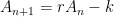
In the past few posts, we have considered the solution of the following recurrence relation, which is often used to model the payment of a mortgage or of credit-card debt:
With this difference equation, the rate at which the principal is reduced can be simply computed using Microsoft Excel. This tool is called an amortization schedule or an amortization table; see E-How for the instructions of how to build one. Here’s a sample Excel spreadsheet that I’ll be illustrating below: Amortization schedule. My personal experience is that many math majors have never seen such a spreadsheet, even though they are familiar with compound interest problems and certainly have the mathematical tools to understand this spreadsheet.
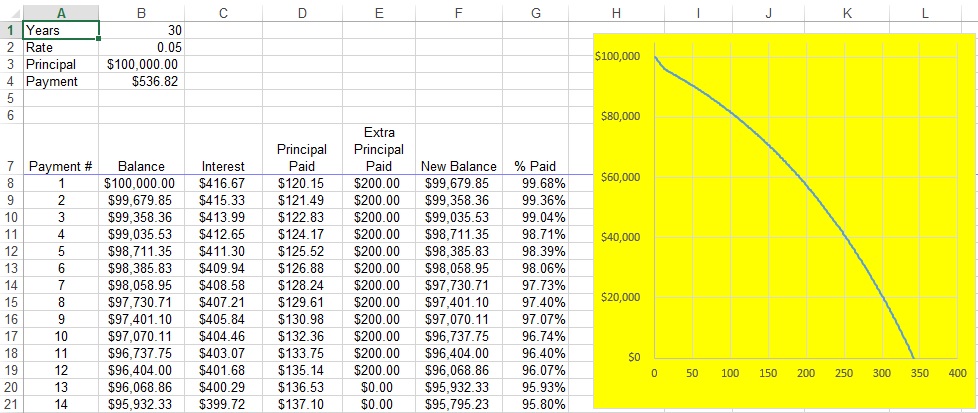
Here’s a screen capture from the spreadsheet:
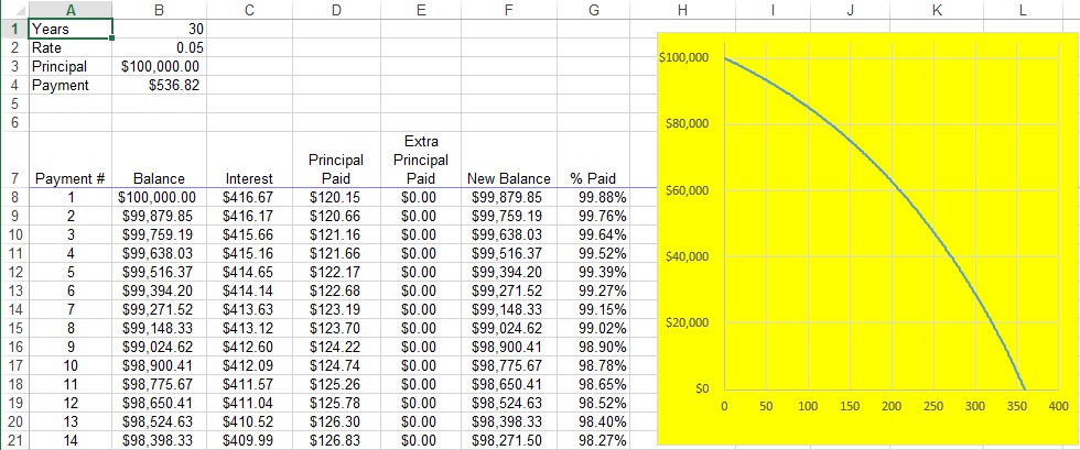
The terms of the loan are typed into Cells B1 (length of loan, in years), B2 (annual percentage rate), and B3 (initial principal). Cell B4 is computed from this information using the Microsoft Excel command  :
:

This is the amount that must be paid every month in order to pay off the loan in the prescribed number of years. Of course, there is a formula for this:
![M = \displaystyle \frac{Pr}{12 \displaystyle \left[1 - \left( 1 + \frac{r}{12} \right)^{-12t} \right]}](https://s0.wp.com/latex.php?latex=M+%3D+%5Cdisplaystyle+%5Cfrac%7BPr%7D%7B12+%5Cdisplaystyle+%5Cleft%5B1+-+%5Cleft%28+1+%2B+%5Cfrac%7Br%7D%7B12%7D+%5Cright%29%5E%7B-12t%7D+%5Cright%5D%7D&bg=ffffff&fg=000000&s=0&c=20201002)
I won’t go into the derivation of this formula here, as it’s a bit complicated. Notice that this formula does not include escrow, points, closing costs, etc. This is strictly the amount of money that’s needed to pay down the principal.
The table, beginning in Row 8 of the above picture, shows how quickly the principal will be paid off. In row 8, the interest that’s paid for that month is computed by
Therefore, the amount of the monthly payment that actually goes toward paying down the principal will be

Column E provides an opportunity to pay something extra each month; more on this later. So, after taking into account the payments in columns D and E, the amount remaining on the loan is recorded in Cell F8:
This amount is then copied into Cell B9, and then the pattern can be filled down.
The yellow graph shows how quickly the balance of the loan is paid off over the length of the loan. A picture is worth a thousand words: in the initial years of the loan, most of the payments are gobbled up by the interest, and so the principal is paid off slowly. Only in the latter years of the loan is the principal paid off quickly.
So, it stands to reason that any extra payments in the initial months and years of the loan can do wonders for paying off the loan quickly. For example, here’s a screenshot of what happens if an extra $200/month is paid only in the first 12 months of the loan:
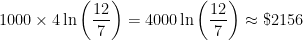
 A definite bend in the graph is evident in the initial 12 months until the normal payment is resumed in month 13. As a result of those extra payments, the curve now intersects the horizontal axis around 340. In other words, 20 fewer months are required to pay off the loan. Stated another way, the extra payments in the first year cost an extra
  . However, in the long run, those payments saved about
  !
!


 (which is greater than 1), and from this product the amount paid is deducted. With this approach — and unlike the approach using calculus — the payment period would be each month and not per year. Therefore, we can write
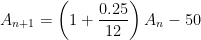


 in Cell A2 and
  in Cell B2. (In the screenshot below, I changed the format of column B to show dollars and cents.) Next, I entered
  in Cell A3 and
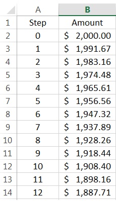


 and looking for a pattern.
 ,
, and
and  are unknown constants.Why do we guess the solution to have this form? I won’t dive into the details, but this is entirely analogous to constructing
  instead of
  , we find that
 .
.


 :
:


 .
. and solve for

![0 = r^n \left( P[1-r] + k \right) - k](https://s0.wp.com/latex.php?latex=0+%3D+r%5En+%5Cleft%28+P%5B1-r%5D+%2B+k+%5Cright%29+-+k&bg=ffffff&fg=000000&s=0&c=20201002)
![k = r^n \left( P[1-r] + k \right)](https://s0.wp.com/latex.php?latex=k+%3D+r%5En+%5Cleft%28+P%5B1-r%5D+%2B+k+%5Cright%29&bg=ffffff&fg=000000&s=0&c=20201002)
![\displaystyle \frac{k}{P[1-r] + k} = r^n](https://s0.wp.com/latex.php?latex=%5Cdisplaystyle+%5Cfrac%7Bk%7D%7BP%5B1-r%5D+%2B+k%7D+%3D+r%5En&bg=ffffff&fg=000000&s=0&c=20201002)
![\displaystyle \ln \left( \frac{k}{P[1-r]+k} \right) = n \ln r](https://s0.wp.com/latex.php?latex=%5Cdisplaystyle+%5Cln+%5Cleft%28+%5Cfrac%7Bk%7D%7BP%5B1-r%5D%2Bk%7D+%5Cright%29+%3D+n+%5Cln+r&bg=ffffff&fg=000000&s=0&c=20201002)
![\displaystyle \frac{ \displaystyle \ln \left( \frac{k}{P[1-r]+k} \right) }{ \ln r} = n](https://s0.wp.com/latex.php?latex=%5Cdisplaystyle+%5Cfrac%7B+%5Cdisplaystyle+%5Cln+%5Cleft%28+%5Cfrac%7Bk%7D%7BP%5B1-r%5D%2Bk%7D+%5Cright%29+%7D%7B+%5Cln+r%7D+%3D+n&bg=ffffff&fg=000000&s=0&c=20201002)
 ,
,  , and
, and  :
: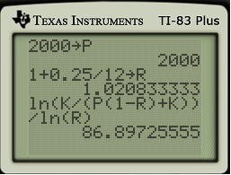
 years, which is nearly equal to the value of
  years
years  , we find
 .
. , we find


 , we find
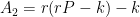
![A_3 = r \left[ r^2 P - k(1+r) \right] - k](https://s0.wp.com/latex.php?latex=A_3+%3D+r+%5Cleft%5B+r%5E2+P+-+k%281%2Br%29+%5Cright%5D+-+k&bg=ffffff&fg=000000&s=0&c=20201002)


 ,
,  , and
, and  years is
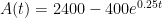 .
.

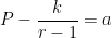
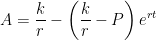
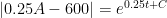
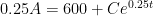
 , has solution
 is the initial amount,
  is the amount paid per year. In other words, students could be given the formula without the full explanation of where it comes from. After all, many Precalculus textbooks give the formula for Newton’s Law of Cooling (the subject of a future post) with neither derivation nor explanation (though its derivation is nearly identical to the work of yesterday’s post), So I don’t see why also giving students the above formula for paying off credit-card debt isn’t more common.
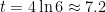 years to pay off the debt.
 per year for
  years, and so the amount spent is
 .
.
 :
:


 .
. be the amount of money on the credit card after
  per year.
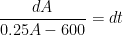


 , we use the initial condition


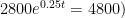
 . As part of this series, we considered the formula for continuous compound interest
 with solution
  . The meaning of the value of
  are
are  , while the units of
  . Therefore, the units of
  . So saying that there’s a “relative rate of growth of 10% per hour” makes total sense.
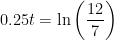
 .” But this is a horrible way to write this in ordinary English! After all, if we plug
  into the formula, we obtain


