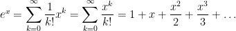
I’m in the middle of a series of posts describing how I remind students about Taylor series. In the previous posts, I described how I lead students to the definition of the Maclaurin series

which converges to 

Step 4. Let’s now get some practice with Maclaurin series. Let’s start with 
What’s 

Next, to find 


How about 


Plugging into the above formula, we find that
It turns out that the radius of convergence for this power series is 

At this point, students generally feel confident about the mechanics of finding a Taylor series expansion, and that’s a good thing. However, in my experience, their command of Taylor series is still somewhat artificial. They can go through the motions of taking derivatives and finding the Taylor series, but this complicated symbol in 
So I shift gears somewhat to discuss the rate of convergence. My hope is to deepen students’ knowledge by getting them to believe that
Pedagogically, I like to use a spreadsheet like Microsoft Excel to demonstrate the rate of convergence. A calculator could be used, but students can see quickly with Excel how quickly (or slowly) the terms get smaller. I usually construct the spreadsheet in class on the fly (the fill down feature is really helpful for doing this quickly), with the end product looking something like this:

In this way, students can immediately see that the Taylor series is accurate to four significant digits by going up to the 
In short, this is how a calculator computes 
Then I shift gears by trying a larger value of
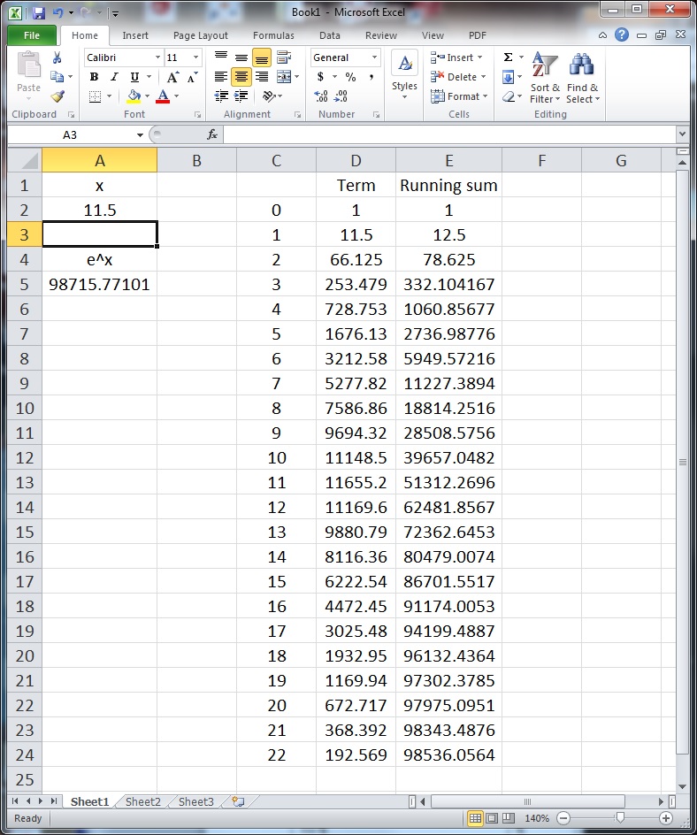
I ask my students the obvious question: What went wrong? They’re usually able to volunteer a few ideas:
- The convergence is slower for larger values of
- The series will converge, but more terms are needed (and I’ll later use the fill down feature to get enough terms so that it does converge as accurate as double precision will allow).
- The individual terms get bigger until
and then start getting smaller. I’ll ask my students why this happens, and I’ll eventually get an explanation like

but

At this point, I’ll mention that calculators use some tricks to speed up convergence. For example, the calculator can simply store a few values of 


The first three values don’t need to be computed — they’ve already been stored in memory — while the last value can be computed via Taylor series. Also, since 


At this point — after doing these explicit numerical examples — I’ll show graphs of
At this point, I hope my students are familiar with the definition of Taylor (Maclaurin) series, can apply the definition to
In the next post, we’ll consider another Taylor series which ought to be (but usually isn’t) really familiar to students: an infinite geometric series.
P.S. Here’s the Excel spreadsheet that I used to make the above figures: Taylor.

13 thoughts on “Reminding students about Taylor series (Part 4)”