Sadly, at least at my university, Taylor series is the topic that is least retained by students years after taking Calculus II. They can remember the rules for integration and differentiation, but their command of Taylor series seems to slip through the cracks. In my opinion, the reason for this lack of retention is completely understandable from a student’s perspective: Taylor series is usually the last topic covered in a semester, and so students learn them quickly for the final and quickly forget about them as soon as the final is over.
Of course, when I need to use Taylor series in an advanced course but my students have completely forgotten this prerequisite knowledge, I have to get them up to speed as soon as possible. Here’s the sequence that I use to accomplish this task. Covering this sequence usually takes me about 30 minutes of class time.
I should emphasize that I present this sequence in an inquiry-based format: I ask leading questions of my students so that the answers of my students are driving the lecture. In other words, I don’t ask my students to simply take dictation. It’s a little hard to describe a question-and-answer format in a blog, but I’ll attempt to do this below.
In the previous posts, I described how I lead students to the definition of the Maclaurin series
 ,
,
which converges to  within some radius of convergence for all functions that commonly appear in the secondary mathematics curriculum.

Step 7. Let’s now turn to trigonometric functions, starting with  .
.
What’s  ? Plugging in, we find
  .
.
As before, we continue until we find a pattern. Next,  , so that
  .
.
Next,  , so that
  .
.
Next,  , so that
  .
.
No pattern yet. Let’s keep going.
Next,  , so that
  .
.
Next,  , so that
  .
.
Next,  , so that
  .
.
Next,  , so that
  .
.
OK, it looks like we have a pattern… albeit more awkward than the patterns for  and
and  . Plugging into the series, we find that
If we stare at the pattern of terms long enough, we can write this more succinctly as

The  term accounts for the alternating signs (starting on positive with
  ), while the
  is needed to ensure that each exponent and factorial is odd.
Let’s see…  has a Taylor expansion that only has odd exponents. In what other sense are the words “sine” and “odd” associated?
In Precalculus, a function is called odd if  for all numbers
  . For example,
  is odd since
  since 9 is a (you guessed it) an odd number. Also,
  , and so is also an odd function. So we shouldn’t be that surprised to see only odd exponents in the Taylor expansion of .
A pedagogical note: In my opinion, it’s better (for review purposes) to avoid the  notation and simply use the “dot, dot, dot” expression instead. The point of this exercise is to review a topic that’s been long forgotten so that these Taylor series can be used for other purposes. My experience is that the adds a layer of abstraction that students don’t need to overcome for the time being.
Step 8. Let’s now turn try  .
.
What’s ? Plugging in, we find  .
.
Next,  , so that
  .
.
Next,  , so that
  .
.
It looks like the same pattern of numbers as above, except shifted by one derivative. Let’s keep going.
Next,  , so that
  .
.
Next,  , so that
  .
.
Next,  , so that
  .
.
Next,  , so that
  .
.
OK, it looks like we have a pattern somewhat similar to that of $\sin x$, except only involving the even terms. I guess that shouldn’t be surprising since, from precalculus we know that  is an even function since
  for all .
Plugging into the series, we find that

If we stare at the pattern of terms long enough, we can write this more succinctly as

As we saw with , the above series converge quickest for values of near  . In the case of and , this may be facilitated through the use of trigonometric identities, thus accelerating convergence.
For example, the series for  will converge quite slowly (after converting
  into radians). However, we know that

using the periodicity of . Next, since $\latex 280^o$ is in the fourth quadrant, we can use the reference angle to find an equivalent angle in the first quadrant:

Finally, using the cofunction identity  , we find
 .
.
In this way, the sine or cosine of any angle can be reduced to the sine or cosine of some angle between  and $45^o = \pi/4$ radians. Since
  , the above power series will converge reasonably rapidly.
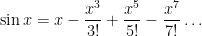
Step 10. For the final part of this review, let’s take a second look at the Taylor series
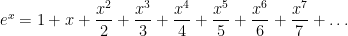
Just to be silly — for no apparent reason whatsoever, let’s replace by  and see what happens:
![e^{ix} = \displaystyle 1 - \frac{x^2}{2!} + \frac{x^4}{4!} - \frac{x^6}{6!} \dots + i \left[\displaystyle x - \frac{x^3}{3!} + \frac{x^5}{5!} - \frac{x^7}{7!} \dots \right]](https://s0.wp.com/latex.php?latex=e%5E%7Bix%7D+%3D+%5Cdisplaystyle+1+-+%5Cfrac%7Bx%5E2%7D%7B2%21%7D+%2B+%5Cfrac%7Bx%5E4%7D%7B4%21%7D+-+%5Cfrac%7Bx%5E6%7D%7B6%21%7D+%5Cdots+%2B+i+%5Cleft%5B%5Cdisplaystyle+x+-+%5Cfrac%7Bx%5E3%7D%7B3%21%7D+%2B+%5Cfrac%7Bx%5E5%7D%7B5%21%7D+-+%5Cfrac%7Bx%5E7%7D%7B7%21%7D+%5Cdots+%5Cright%5D&bg=ffffff&fg=000000&s=0&c=20201002)
after separating the terms that do and don’t have an  .
.
Hmmmm… looks familiar….
So it makes sense to define
 ,
,
which is called Euler’s formula, thus proving an unexpected connected between and the trigonometric functions.

 .
. .
. , we first find
  . Using the Chain Rule, we find
  , so that
  , so that
  .
. , so that
  .
. , so that
  .
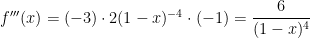
. , and this can be formally proved by induction.
 .
. . Unlike the series for
  .
.
 and $r=x$. Also, as stated in precalculus, this series only converges if the common ratio satisfies $|r| < 1$, as before.
 ,
, .
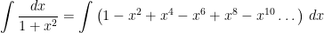
. in the Taylor series in Step 5, obtaining


 :
:

 can be found by replacing

 in the Taylor series in Step 5, obtaining
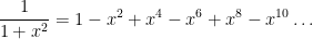


 .
. .
. . So
. So  .
. ? Yep, it’s also
  for all
  , though we’ll skip the formal proof by induction.
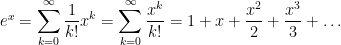
 . In other words, the series on the right converges for all values of
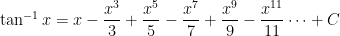
 term and that about ten or eleven terms are needed to get a figure that is as accurate as the
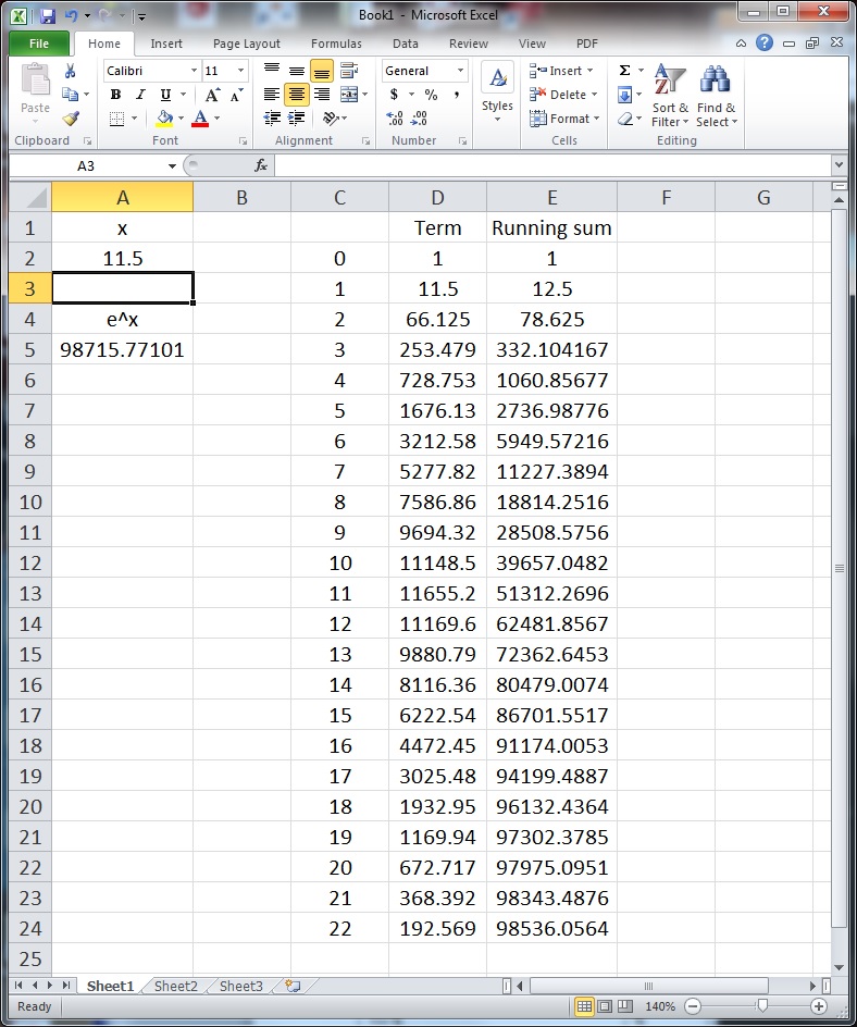
 and then start getting smaller. I’ll ask my students why this happens, and I’ll eventually get an explanation like

 ,
,  ,
,  ,
,  , and
, and  . I then ask my class how these could be used to find
  . After some thought, they will volunteer that
 .
. , the series for
  will converge pretty quickly. (Some students may volunteer that the above product is logically equivalent to turning
  into binary.)
 .
. ,
, can be any number.
 .
. .
. .
. , which is so “flat” near $x=0$ that every single derivative of
  .
. is the
  coordinate at
  .
. is the slope of the curve at
  is a measure of the concavity of the curve at — you guessed it —
  is an even more subtle description of the curve… once again, at
  ,
,  ,
,  ,
,  , and
, and  .
. , and start differentiating. Remember that
  ,
,  ,
,  , and
, and  are constants.
 . Therefore, it must be that
  .
. , and so
  . Since
  .
. , and so
  . Since
  , or
, or  .
. , and so
  . Since
  , or
, or  .
. , and so
  . Since
  , or
, or  .
. .
. by
by  . Where did the
  , and so
 .
. by
by  . The number
  , and so
 .
. .
. and
and  .
. and
and  .
. .
. term has a coefficient involving the third derivative of
  and the last term is multiplied by
  .
. where have we seen those before? Oh yes, the
  ,
,  ,
,  ,
,  , and
, and  is defined to be
  .
. notation:
 .
. A good working knowledge of Taylor series is necessary for computing series solutions of ordinary differential equations.
 are used over and over again. For example, the
 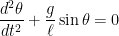 ,
, is the acceleration due to gravity and
  is the length of the pendulum. This differential equation cannot be solved exactly, and its solution is
  , so that the differential equation becomes
 ,
, term, we now have a second-order differential equation with constant coefficients, which can be solved in a straightforward manner using standard techniques from differential equations. If
  and
and  (i.e., the pendulum is pulled a small angle
  and is then released), the solution is
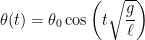 .
. coordinate of the terminal point. Instead, the calculator converts
 , and (as I’ll discuss) the Maclaurin series for
  converges much faster than the Maclaurin series for
  .
. Height restriction)
 160 cm) The world’s largest hockey stick and puck are in Duncan, British Columbia. The stick is over 62 m in length and weighs almost 28,000 kg. Is your equipment legal?
