Dr. Matthew Weathers is an assistant professor of Mathematics and Computer Science at Biola University and also a world-class showman. Here are some of his biggest hits (often for Halloween or April Fools’ Day). Enjoy. (If you’re interested, you can find more at his YouTube page, http://www.youtube.com/user/MDWeathers/videos?sort=p&view=0&flow=grid.
Author: John Quintanilla
I'm a Professor of Mathematics and a University Distinguished Teaching Professor at the University of North Texas. For eight years, I was co-director of Teach North Texas, UNT's program for preparing secondary teachers of mathematics and science.
Geometric magic trick
This is a magic trick that my math teacher taught me when I was about 13 or 14. I’ve found that it’s a big hit when performed for grade-school children.
Magician: Tell me a number between 3 and 10.
Child: (gives a number, call it
)
Magician: On a piece of paper, draw a shape with
Child: (draws a figure; an example for
is shown)
Important Note: For this trick to work, the original shape has to be convex… something shaped like an L or M won’t work. Also, I chose a maximum of 10 mostly for ease of drawing and counting (and, for later, calculating).
Magician: Tell me another number between 3 and 10.
Child: (gives a number, call it
)
Magician: Now draw that many dots inside of your shape.
Child: (starts drawing
) While the child does this, the Magician calculates
, writes the answer on a piece of paper, and turns the answer face down.
Magician: Now connect the dots with lines until you get all triangles. Just be sure that no two lines cross each other.
Child: (connects the dots until the shape is divided into triangles; an example is shown)
Magician: Now count the number of triangles.
Child: (counts the triangles)
Magician: Was your answer… (and turns the answer over)?


The reason this magic trick works so well is that it’s so counter-intuitive. No matter what convex 


Why does this magic trick work? I offer a thought bubble if you’d like to think about it before scrolling down to see the answer.
 This trick works by counting the measures of all the angles in two different ways.
Method #1: If there are 


 Method #2: The sum of the measures of the angles around each interior point is

 The measures of the remaining angles add up to the sum of the measures of the interior angles of a convex polygon with
 In other words, it must be the case that


Welch’s formula
When conducting an hypothesis test or computing a confidence interval for the difference 

rounded down to the nearest integer. In this formula, 


The terms 


In Welch’s formula, the term 


This leads to the “Pythagorean” relationship

which (in my experience) is a reasonable aid to help students remember the formula for

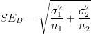
Naturally, a big problem that students encounter when using Welch’s formula is that the formula is really, really complicated, and it’s easy to make a mistake when entering information into their calculators. (Indeed, it might be that the pre-programmed calculator function simply gives the wrong answer.) Also, since the formula is complicated, students don’t have a lot of psychological reassurance that, when they come out the other end, their answer is actually correct. So, when teaching this topic, I tell my students the following rule of thumb so that they can at least check if their final answer is plausible:

To my surprise, I have never seen this formula in a statistics textbook, even though it’s quite simple to state and not too difficult to prove using techniques from first-semester calculus.
Let’s rewrite Welch’s formula as
![df = \left( \displaystyle \frac{1}{n_1-1} \left[ \frac{SE_1^2}{SE_1^2 + SE_2^2}\right]^2 + \frac{1}{n_2-1} \left[ \frac{SE_2^2}{SE_1^2 + SE_2^2} \right]^2 \right)^{-1}](https://s0.wp.com/latex.php?latex=df+%3D+%5Cleft%28+%5Cdisplaystyle+%5Cfrac%7B1%7D%7Bn_1-1%7D+%5Cleft%5B+%5Cfrac%7BSE_1%5E2%7D%7BSE_1%5E2+%2B+SE_2%5E2%7D%5Cright%5D%5E2+%2B+%5Cfrac%7B1%7D%7Bn_2-1%7D+%5Cleft%5B+%5Cfrac%7BSE_2%5E2%7D%7BSE_1%5E2+%2B+SE_2%5E2%7D+%5Cright%5D%5E2+%5Cright%29%5E%7B-1%7D&bg=ffffff&fg=000000&s=0&c=20201002)
For the sake of simplicity, let 

![df = \left( \displaystyle \frac{1}{m_1} \left[ \frac{SE_1^2}{SE_1^2 + SE_2^2}\right]^2 + \frac{1}{m_2} \left[ \frac{SE_2^2}{SE_1^2 + SE_2^2} \right]^2 \right)^{-1}](https://s0.wp.com/latex.php?latex=df+%3D+%5Cleft%28+%5Cdisplaystyle+%5Cfrac%7B1%7D%7Bm_1%7D+%5Cleft%5B+%5Cfrac%7BSE_1%5E2%7D%7BSE_1%5E2+%2B+SE_2%5E2%7D%5Cright%5D%5E2+%2B+%5Cfrac%7B1%7D%7Bm_2%7D+%5Cleft%5B+%5Cfrac%7BSE_2%5E2%7D%7BSE_1%5E2+%2B+SE_2%5E2%7D+%5Cright%5D%5E2+%5Cright%29%5E%7B-1%7D&bg=ffffff&fg=000000&s=0&c=20201002)
Now let 


Using these observations, Welch’s formula reduces to the function
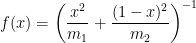
and the central problem is to find the maximum and minimum values of 

![[0,1]](https://s0.wp.com/latex.php?latex=%5B0%2C1%5D&bg=ffffff&fg=000000&s=0&c=20201002)
First, the endpoints. If 


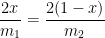
Next, the critical point(s). These are found by solving the equation 
![f'(x) = -\left( \displaystyle \frac{x^2}{m_1} + \frac{(1-x)^2}{m_2} \right)^{-2} \left[ \displaystyle \frac{2x}{m_1} - \frac{2(1-x)}{m_2} \right] = 0](https://s0.wp.com/latex.php?latex=f%27%28x%29+%3D+-%5Cleft%28+%5Cdisplaystyle+%5Cfrac%7Bx%5E2%7D%7Bm_1%7D+%2B+%5Cfrac%7B%281-x%29%5E2%7D%7Bm_2%7D+%5Cright%29%5E%7B-2%7D+%5Cleft%5B+%5Cdisplaystyle+%5Cfrac%7B2x%7D%7Bm_1%7D+-+%5Cfrac%7B2%281-x%29%7D%7Bm_2%7D+%5Cright%5D+%3D+0&bg=ffffff&fg=000000&s=0&c=20201002)

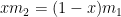


Plugging back into the original equation, we find the local extremum
![f \left( \displaystyle \frac{m_1}{m_1+m_2} \right) = \left( \displaystyle \frac{1}{m_1} \frac{m_1^2}{(m_1+m_2)^2} + \frac{1}{m_2} \left[1-\frac{m_1}{m_1+m_2}\right]^2 \right)^{-1}](https://s0.wp.com/latex.php?latex=f+%5Cleft%28+%5Cdisplaystyle+%5Cfrac%7Bm_1%7D%7Bm_1%2Bm_2%7D+%5Cright%29+%3D+%5Cleft%28+%5Cdisplaystyle+%5Cfrac%7B1%7D%7Bm_1%7D+%5Cfrac%7Bm_1%5E2%7D%7B%28m_1%2Bm_2%29%5E2%7D+%2B+%5Cfrac%7B1%7D%7Bm_2%7D+%5Cleft%5B1-%5Cfrac%7Bm_1%7D%7Bm_1%2Bm_2%7D%5Cright%5D%5E2+%5Cright%29%5E%7B-1%7D&bg=ffffff&fg=000000&s=0&c=20201002)
![f \left( \displaystyle \frac{m_1}{m_1+m_2} \right) = \left( \displaystyle \frac{1}{m_1} \frac{m_1^2}{(m_1+m_2)^2} + \frac{1}{m_2} \left[\frac{m_2}{m_1+m_2}\right]^2 \right)^{-1}](https://s0.wp.com/latex.php?latex=f+%5Cleft%28+%5Cdisplaystyle+%5Cfrac%7Bm_1%7D%7Bm_1%2Bm_2%7D+%5Cright%29+%3D+%5Cleft%28+%5Cdisplaystyle+%5Cfrac%7B1%7D%7Bm_1%7D+%5Cfrac%7Bm_1%5E2%7D%7B%28m_1%2Bm_2%29%5E2%7D+%2B+%5Cfrac%7B1%7D%7Bm_2%7D+%5Cleft%5B%5Cfrac%7Bm_2%7D%7Bm_1%2Bm_2%7D%5Cright%5D%5E2+%5Cright%29%5E%7B-1%7D&bg=ffffff&fg=000000&s=0&c=20201002)


Based on the three local extrema that we’ve found, it’s clear that the absolute minimum of 


In conclusion, I suggest offering the following guidelines to students to encourage their intuition about the plausibility of their answers:
- If
is much smaller than
), then
will be close to
.
- If
), then
- Otherwise,
, but no larger.
Statistical significance
When teaching my Applied Statistics class, I’ll often use the following xkcd comic to reinforce the meaning of statistical significance.

The idea that’s being communicated is that, when performing an hypothesis test, the observed significance level 

In practice, statisticians use the Bonferroni correction when performing multiple simultaneous tests to avoid the erroneous conclusion displayed in the comic.
Source: http://www.xkcd.com/882/
Engaging students in a different discipline
I have no expertise about how to teach any other subject besides mathematics. But this article from the May/June 2013 issue of the Stanford alumni magazine made a lot of sense to me about how to teach history to middle- and high-school students. The basic principle appears to be the same that governs my classes: figure out a way to make students want to come to class each day. A sample quote:
I easily could have told them in one minute that the Dust Bowl was the result of overgrazing and over-farming and World War I overproduction, combined with droughts that had been plaguing that area forever, but they wouldn’t remember it.” By reading these challenging documents and discovering history for themselves, he says, “not only will they remember the content, they’ll develop skills for life.
For history, the widespread implementation of this teaching philosophy has apparently been hindered by the lack of adequate teaching materials, which is also addressed in this article.
Dimensions
As described by the March 2013 issue of the American Mathematical Monthly, the (free!) two-hour movie Dimensions is “an impressive computer-generated video of almost 2 hours that describes geometry in two, three and four dimensions. The video assumes an elementary geometry background possessed by most viewers and leads up to an interesting geometric structure, the Hopf fibration of the unit sphere in four-dimensional space.”
The website of this project can be found at http://www.dimensions-math.org.
Here’s the 4-minute trailer for the movie:
This full two-hour movie was uploaded to YouTube in several chapters. The full YouTube playlist is given here.
The links to the 9 separate chapters are below.
Circular logic
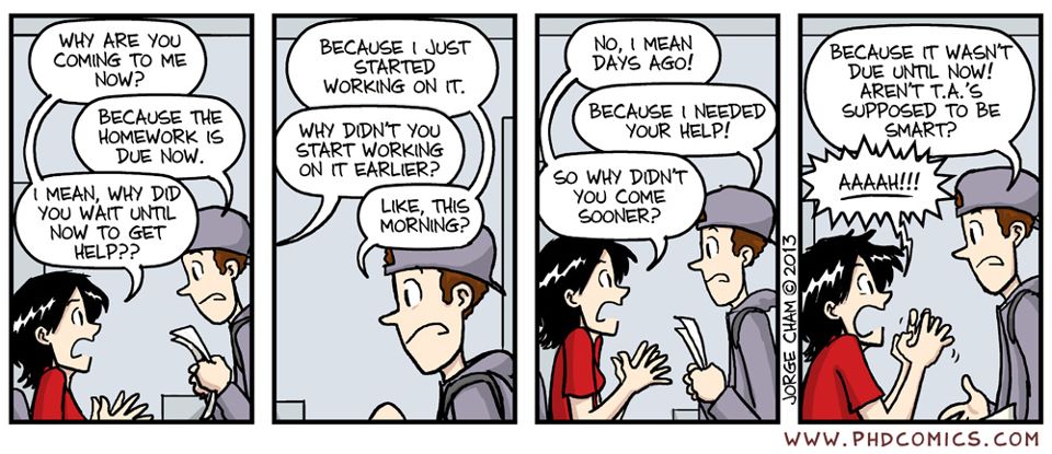
What makes my blood boil
A friend of mine forwarded the following image to me on Facebook:
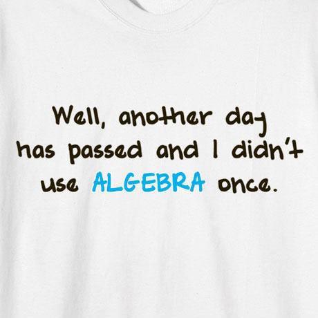
My response was quick and simple: Anybody who’s able to use a computer or a mobile device to use Facebook to connect with their friends has directly benefited from algebra today, whether or not they realize it.
Put Understanding First
From a great article by G. Wiggins and J. McTighe, “Put Understanding First,” Reshaping High Schools, Vol. 65, No. 8, pp. 36-41 (May 2008)
Out-of-context learning of skills is arguably one of the greatest weaknesses of the secondary curriculum—the natural outgrowth of marching through the textbook instead of teaching with meaning and transfer in mind. Schools too often teach and test mathematics, writing, and world language skills in isolation rather than in the context of authentic demands requiring thoughtful application. If we don’t give students sufficient ongoing opportunities to puzzle over genuine problems, make meaning of their learning, and apply content in various contexts, then long-term retention and effective performance are unlikely, and high schools will have failed to achieve their purpose.
A cute mathematical challenge
Show each number from 0 to 25 as a combination of four 
For example: 
