Square roots and logarithms without a calculator (Part 10)

This is the fifth in a series of posts about calculating roots without a calculator, with special consideration to how these tales can engage students more deeply with the secondary mathematics curriculum. As most students today have a hard time believing that square roots can be computed without a calculator, hopefully giving them some appreciation for their elders.

Today’s story takes us back to a time before the advent of cheap pocket calculators: 1949.

The following story comes from the chapter “Lucky Numbers” of Surely You’re Joking, Mr. Feynman!, a collection of tales by the late Nobel Prize winning physicist, Richard P. Feynman. Feynman was arguably the greatest American-born physicist — the subject of the excellent biography Genius: The Life and Science of Richard Feynman — and he had a tendency to one-up anyone who tried to one-up him. (He was also a serial philanderer, but that’s another story.) Here’s a story involving how, in the summer of 1949, he calculated $\sqrt[3]{1729.03}$ without a calculator.

The first time I was in Brazil I was eating a noon meal at I don’t know what time — I was always in the restaurants at the wrong time — and I was the only customer in the place. I was eating rice with steak (which I loved), and there were about four waiters standing around.

A Japanese man came into the restaurant. I had seen him before, wandering around; he was trying to sell abacuses. (Note: At the time of this story, before the advent of pocket calculators, the abacus was arguably the world’s most powerful hand-held computational device.) He started to talk to the waiters, and challenged them: He said he could add numbers faster than any of them could do.

The waiters didn’t want to lose face, so they said, “Yeah, yeah. Why don’t you go over and challenge the customer over there?”

The man came over. I protested, “But I don’t speak Portuguese well!”

The waiters laughed. “The numbers are easy,” they said.

They brought me a paper and pencil.

The man asked a waiter to call out some numbers to add. He beat me hollow, because while I was writing the numbers down, he was already adding them as he went along.

I suggested that the waiter write down two identical lists of numbers and hand them to us at the same time. It didn’t make much difference. He still beat me by quite a bit.

However, the man got a little bit excited: he wanted to prove himself some more. “Multiplição!” he said.

Somebody wrote down a problem. He beat me again, but not by much, because I’m pretty good at products.

The man then made a mistake: he proposed we go on to division. What he didn’t realize was, the harder the problem, the better chance I had.

We both did a long division problem. It was a tie.

This bothered the hell out of the Japanese man, because he was apparently well trained on the abacus, and here he was almost beaten by this customer in a restaurant.

“Raios cubicos!” he says with a vengeance. Cube roots! He wants to do cube roots by arithmetic. It’s hard to find a more difficult fundamental problem in arithmetic. It must have been his topnotch exercise in abacus-land.

He writes down a number on some paper— any old number— and I still remember it: $1729.03$ . He starts working on it, mumbling and grumbling: “Mmmmmmagmmmmbrrr”— he’s working like a demon! He’s poring away, doing this cube root.

Meanwhile I’m just sitting there.

One of the waiters says, “What are you doing?”.

I point to my head. “Thinking!” I say. I write down $12$ on the paper. After a little while I’ve got $12.002$ .

The man with the abacus wipes the sweat off his forehead: “Twelve!” he says.

“Oh, no!” I say. “More digits! More digits!” I know that in taking a cube root by arithmetic, each new digit is even more work that the one before. It’s a hard job.

He buries himself again, grunting “Rrrrgrrrrmmmmmm …,” while I add on two more digits. He finally lifts his head to say, “ $12.0$ !”

The waiter are all excited and happy. They tell the man, “Look! He does it only by thinking, and you need an abacus! He’s got more digits!”

He was completely washed out, and left, humiliated. The waiters congratulated each other.

How did the customer beat the abacus?

The number was $1729.03$ . I happened to know that a cubic foot contains $1728$ cubic inches, so the answer is a tiny bit more than $12$ . The excess, $1.03$ , is only one part in nearly $2000$ , and I had learned in calculus that for small fractions, the cube root’s excess is one-third of the number’s excess. So all I had to do is find the fraction $1/1728$ , and multiply by $4$ (divide by $3$ and multiply by $12$ ). So I was able to pull out a whole lot of digits that way.

A few weeks later, the man came into the cocktail lounge of the hotel I was staying at. He recognized me and came over. “Tell me,” he said, “how were you able to do that cube-root problem so fast?”

I started to explain that it was an approximate method, and had to do with the percentage of error. “Suppose you had given me $28$ . Now the cube root of $27$ is $3$ …”

He picks up his abacus: zzzzzzzzzzzzzzz— “Oh yes,” he says.

I realized something: he doesn’t know numbers. With the abacus, you don’t have to memorize a lot of arithmetic combinations; all you have to do is to learn to push the little beads up and down. You don’t have to memorize 9+7=16; you just know that when you add 9, you push a ten’s bead up and pull a one’s bead down. So we’re slower at basic arithmetic, but we know numbers.

Furthermore, the whole idea of an approximate method was beyond him, even though a cubic root often cannot be computed exactly by any method. So I never could teach him how I did cube roots or explain how lucky I was that he happened to choose $1729.03$ .

The key part of the story, “for small fractions, the cube root’s excess is one-third of the number’s excess,” deserves some elaboration, especially since this computational trick isn’t often taught in those terms anymore. If $f(x) = (1+x)^n$ , then $f'(x) = n (1+x)^{n-1}$ , so that $f'(0) = n$ . Since $f(0) = 1$ , the equation of the tangent line to $f(x)$ at $x = 0$ is

$L(x) = f(0) + f'(0) \cdot (x-0) = 1 + nx$ .

The key observation is that, for $x \approx 0$ , the graph of $L(x)$ will be very close indeed to the graph of $f(x)$ . In Calculus I, this is sometimes called the linearization of $f$ at $x =a$ . In Calculus II, we observe that these are the first two terms in the Taylor series expansion of $f$ about $x = a$ .

For Feynman’s problem, $n =\frac{1}{3}$ , so that $\sqrt[3]{1+x} \approx 1 + \frac{1}{3} x$ if $x \approx 0$. Then $\latex \sqrt[3]{1729.03}$ can be rewritten as

$\sqrt[3]{1729.03} = \sqrt[3]{1728} \sqrt[3]{ \displaystyle \frac{1729.03}{1728} }$

$\sqrt[3]{1729.03} = 12 \sqrt[3]{\displaystyle 1 + \frac{1.03}{1728}}$

$\sqrt[3]{1729.03} \approx 12 \left( 1 + \displaystyle \frac{1}{3} \times \frac{1.03}{1728} \right)$

$\sqrt[3]{1729.03} \approx 12 + 4 \times \displaystyle \frac{1.03}{1728}$

This last equation explains the line “all I had to do is find the fraction $1/1728$ , and multiply by $4$ .” With enough patience, the first few digits of the correction can be mentally computed since

$\displaystyle \frac{1.03}{500} < \frac{1.03}{432} = 4 \times \frac{1.03}{1728} < \frac{1.03}{400}$

$\displaystyle \frac{1.03 \times 2}{1000} < 4 \times \frac{1.03}{1728} < \frac{1.03 \times 25}{10000}$

$0.00206 < 4 \times \displaystyle \frac{1.03}{1728} < 0.0025075$

So Feynman could determine quickly that the answer was $12.002\hbox{something}$ .

By the way,

$\sqrt[3]{1729.03} \approx 12.00238378\dots$

$\hbox{Estimate} \approx 12.00238426\dots$

So the linearization provides an estimate accurate to eight significant digits. Additional digits could be obtained by using the next term in the Taylor series.

I have a similar story to tell. Back in 1996 or 1997, when I first moved to Texas and was making new friends, I quickly discovered that one way to get odd facial expressions out of strangers was by mentioning that I was a math professor. Occasionally, however, someone would test me to see if I really was a math professor. One guy (who is now a good friend; later, we played in the infield together on our church-league softball team) asked me to figure out $\sqrt{97}$ without a calculator — before someone could walk to the next room and return with the calculator. After two seconds of panic, I realized that I was really lucky that he happened to pick a number close to $100$ . Using the same logic as above,

$\sqrt{97} = \sqrt{100} \sqrt{1 - 0.03} \approx 10 \left(1 - \displaystyle \frac{0.03}{2}\right) = 9.85$ .

Knowing that this came from a linearization and that the tangent line to $y = \sqrt{1+x}$ lies above the curve, I knew that this estimate was too high. But I didn’t have time to work out a correction (besides, I couldn’t remember the full Taylor series off the top of my head), so I answered/guessed $9.849$ , hoping that I did the arithmetic correctly. You can imagine the amazement when someone punched into the calculator to get $9.84886\dots$

Square roots and logarithms without a calculator (Part 9)

This post is not really about finding square roots but continues Part 8 of this series. Continuing the theme of this series, let’s go back in time to when scientific calculators were not invented… say, 1850.

This is a favorite activity that I use when teaching logarithms to precalculus students. I begin by writing the following on the board, in three or four columns:

$\log_{10} 1$

$\log_{10} 2 \approx 0.301$

$\log_{10} 3 \approx 0.477$

$\log_{10} 4$

$\log_{10} 5$

$\log_{10} 6$

$\log_{10} 7$

$\log_{10} 8$

$\log_{10} 9$

$\log_{10} 10$

$\log_{10} 11$

$\log_{10} 12$

$\log_{10} 13$

$\log_{10} 14$

$\log_{10} 15$

$\log_{10} 16$

$\log_{10} 17$

$\log_{10} 18$

$\log_{10} 19$

$\log_{10} 20$

$\log_{10} 30$

$\log_{10} 40$

$\log_{10} 50$

$\log_{10} 60$

$\log_{10} 70$

$\log_{10} 80$

$\log_{10} 90$

$\log_{10} 100$

In other words, I tell the answer to only $\log_{10} 2$ and $\log_{10} 3$ . The challenge: fill in the rest without a calculator.

In my classes, we found these logarithms by large-group discussion. However, there’s no reason why this couldn’t be done by dividing a class into small groups and letting the groups collaborate. Indeed, I suggested this idea to a former student who was struggling to come up with an engaging activity involving logarithms for an Algebra II class that she was about to teach. She took this idea and ran with it, and she told me it was a big hit with her students.

I provide a thought bubble if you’d like to think about it before I give the answers.

Step 1. Three of these values — $1$ , $10$ , and $100$ — can be found exactly since they’re powers of $10$ .

Step 2. Most of the others can be found by using the laws of logarithms for products, quotients, and powers involving $2$ , $3$ , and $10$ . For example,

$\log_{10} 9 = \log_{10} 3^2 = 2 \log_{10} 3 \approx 2 \times 0.477 = 0.954$

$\log_{10} 20 = \log_{10} 2 + \log_{10} 10 = 1.301$

$\log_{10} 5 = \log_{10} 10 - \log_{10} 2 = 0.699$ .

Of this group, usually $\log_{10} 5$ is the hardest for students to recognize.

Step 3 (optional). A few of the logarithms, like $\log_{10} 7$ , cannot be determined in terms of $\log_{10} 2$ and $\log_{10} 3$ . But they can be approximated to reasonable accuracy with a little creativity. For example,

$\log_{10} 7 = \log_{10} \sqrt{49} = \frac{1}{2} \log_{10} 49 \approx \frac{1}{2} \log_{10} 50 = \frac{1}{2} (1.699) = 0.850$ .

For a really good approximation, we use the fact that $7^4 = 2401 \approx 2400$ .

$\log_{10} 7 = \frac{1}{4} \log_{10} 2401 \approx \frac{1}{4} \log_{10} 2400 = \frac{1}{4} (3 \log_{10} 2 + \log_{10} 3 + \log_{10} 100) = 0.845$ .

To approximate $\log_{10} 17$ , we could use the fact that $(16-1) \times (16 + 1) = 16^2-1$ , or $15 \times 17 = 255 \approx 2^8$ . So

$\log_{10} 17 \approx 8 \log_{10} 2 - \log_{10} 15 = 8 \log_{10} 2 - \log_{10} 3 - \log_{10} 5 = 1.232$

Naturally, any and all of the above results can be confirmed with a scientific calculator.

In my opinion, here are some of the pedagogical benefits of the above activity.

1. This activity solidifies students’ knowledge about the laws of logarithms. The laws of logarithms become less abstract, changing from $\log_{10} xy = \log_{10} x + \log_{10} y$ into something more tangible and comfortable, like positive integers.

2. Hopefully the activity will demystify for students the curious decimal expansions when a calculator returns logarithms. In other words, hopefully the above activity will help

3. The activity should promote some understanding of the values of base-10 logarithms. For example, $0 \le \log_{10} x < 1$ for $1 \le x < 10$ and $1 \le \log_{10} x < 2$ for $10 \le x < 100$ .

4. Students should see that, for large $x$ , $\log_{10}(x+1)$ is not much larger than $\log_{10} x$ . This is another way of saying that the graph of $y = \log_{10} x$ increases very slowly as $x$ increases. So this should provide some future intuition for the graphs of logarithmic functions.

5. The values of $\log_{10} 2, \log_{10} 3, \dots, \log_{10} 9$ are used to construct the unevenly-spaced lines and/or tick marks in log-log graphs and log-linear graphs (which are standard plotting options on many scientific calculators).

Square roots and logarithms without a calculator (Part 8)

I’m in the middle of a series of posts concerning the elementary operation of computing a root. This is such an elementary operation because nearly every calculator has a $\sqrt{~~}$ button, and so students today are accustomed to quickly getting an answer without giving much thought to (1) what the answer means or (2) what magic the calculator uses to find roots. I like to show my future secondary teachers a brief history on this topic… partially to deepen their knowledge about what they likely think is a simple concept, but also to give them a little appreciation for their elders.

To begin, let’s again go back to a time before the advent of pocket calculators… say, 1952.

This story doesn’t go back to 1952 but to Boxing Day 2012 (the day after Christmas). For some reason, my daughter — out of the blue — asked me to compute $\sqrt[19]{25727}$ without a calculator. As my daughter adores the ground I walk on — and I want to maintain this state of mind for as long as humanly possible — I had no choice but to comply. So I might as well have been back in 1952.

In the past few posts, I discussed how log tables and slide rules were used by previous generations to perform this calculation. The problem was that all of these tools were in my office and not at home, and hence were not of immediate use.

The good news is that I had a few logarithms memorized:

$\log_{10} 2 \approx 0.301$ , $\log_{10} 3 \approx 0.477$ , $\log_{10} 7 = 0.845$ ,

and $\ln 10 = 2.3$ .

I had the first two logs memorized when I was a child; the third I memorized later. As I’ll describe, the first three logarithms can be used with the laws of logarithms to closely approximate the base-10 logarithm of nearly any number. The last logarithm was important in previous generations for using the change-of-base formula from $\log_{10}$ to $\ln$ . It was also prominently mentioned in the chapter “Lucky Numbers” from a favorite book of my childhood, Surely You’re Joking Mr. Feynman, so I had that memorized as well.

I also knew that $\ln(1+x) \approx x$ for $x = 0$ from the Taylor expansion of $\ln(1+x)$ .

To begin, I first noticed that $25727 \approx 25600$ , and I knew I could get $\log_{10} 25600$ since $25600 = 2^8 \times 100$ . So I started with

$\log_{10} 25727 = \log_{10} \left(100 \times 256 \times \displaystyle \frac{257.27}{256} \right)$

$\log_{10} 25727 \approx \log_{10} 100 + 8 \log_{10} 2 + \log_{10} 1.005$

$\log_{10} 25727 \approx 2 + 8(0.301) + \displaystyle \frac{\ln 1.005}{\ln 10}$

$\log_{10} 25727 \approx 4.408 + \displaystyle \frac{0.005}{2.3}$

$\log_{10} 25727 \approx 4.408 + 0.002$

$\log_{10} 25727 \approx 4.410$

I did all of the above calculations by hand, cutting off after three decimal places (since I had those base-10 logarithms memorized to only three decimal places). Therefore,

$\log_{10} 25727^(1/19) = \displaystyle \frac{1}{19} \log_{10} 25727 \approx \displaystyle \frac{4.410}{19} \approx 0.232$

So, to complete the calculation, I had to find the value of $x$ so that $\log_{10} x = 0.232$ . This was by far the hardest step, since it could only be done by trial and error. I forget exactly what steps I tried, but here’s a sample:

$\log_{10} 2 \approx 0.301$ . Too big.

$\log_{10} 1.5 = \log_{10} \displaystyle \frac{3}{2} = \log_{10} 3 - \log_{10} 2 \approx 0.477 - 0.301 = 0.176$ . Too small.

$\log_{10} 1.6 = \log_{10} \displaystyle \frac{2^4}{10} = 4\log_{10} 2 - \log_{10} 10 \approx 4(0.301) - 1 = 0.203$ . Too small.

$\log_{10} 1.8 = \log_{10} \displaystyle \frac{2 \cdot 3^2}{10} \approx 0.301 + 2(0.477) - 1 = 0.255$ . Too big.

Eventually, I got to

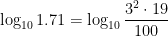
$\log_{10} 1.71 = \log_{10} \displaystyle \frac{3^2 \cdot 19}{100}$

$\log_{10} 1.71 = 2\log_{10} 3 + \log_{10} 19 - \log_{10} 100$

$\log_{10} 1.71 \approx 2(0.477) + \displaystyle \frac{\log_{10} 18 + \log_{10} 20}{2} - 2$

$\log_{10} 1.71 \approx -1.046 + \frac{1}{2} (\log_{10} 2 + 2 \log_{10} 3 + \log_{10} 2 + \log_{10} 10)$

$\log_{10} 1.71 \approx -1.046 + \frac{1}{2}(2.556)$

$\log_{10} 1.71 \approx 0.232$

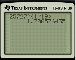
So, after a hour or two of arithmetic, I told her my answer: $\sqrt[19]{25727} \approx 1.71$ . You can imagine my sheer delight when we checked my answer with a calculator:

In Part 9, I’ll discuss my opinion about whether or not these kinds of calculations have any pedagogical value for students learning logarithms.

Square roots and logarithms without a calculator (Part 7)

I’m in the middle of a series of posts concerning the elementary operation of computing a square root. This is such an elementary operation because nearly every calculator has a $\sqrt{~~}$ button, and so students today are accustomed to quickly getting an answer without giving much thought to (1) what the answer means or (2) what magic the calculator uses to find square roots. I like to show my future secondary teachers a brief history on this topic… partially to deepen their knowledge about what they likely think is a simple concept, but also to give them a little appreciation for their elders.

Today’s topic — slide rules — not only applies to square roots but also multiplication, division, and raising numbers to any exponent (not just to the $1/2$ power). To begin, let’s again go back to a time before the advent of pocket calculators… say, the 1950s.

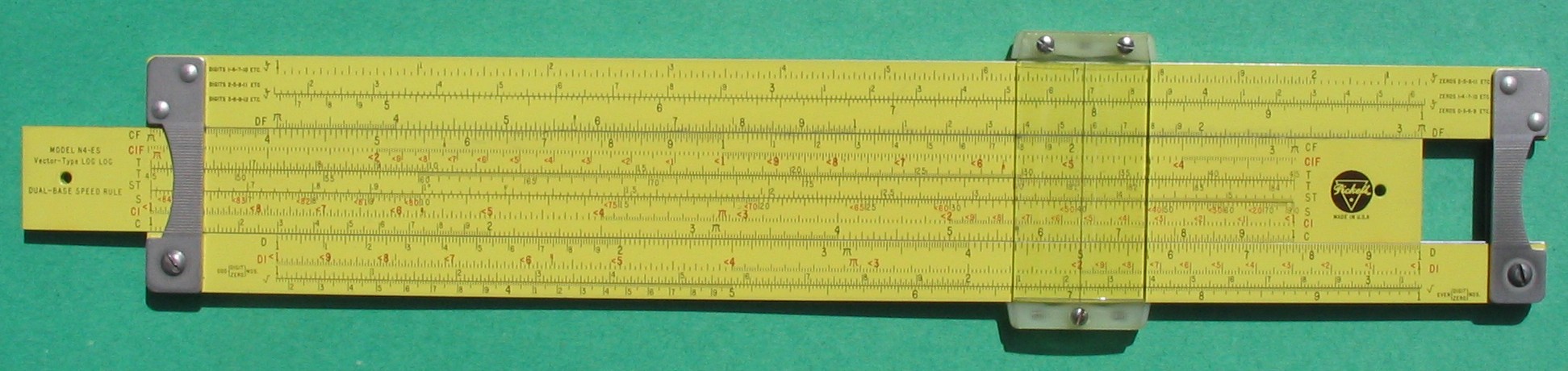
Nearly all STEM professionals were once proficient in the use of slide rules. I never learned how to use one as a student. As a college professor, I bought a fairly inexpensive one from Slide Rule Universe. If you’ve never seen a slide rule, here’s a picture of a fairly advanced one. There are multiple rows of numbers and a sliding plastic piece that has a thin vertical line, allowing direct correspondence from one row of numbers to another. (The middle rows are on a piece that slides back and forth; this is necessary for doing multiplication and division with a slide rule.)

Let’s repeat the problem from Part 6 and try to find

$\log_{10} x = \log_{10} \sqrt{4213} = \log_{10} (4213)^{1/2} = \displaystyle \frac{1}{2} \log_{10} 4213$ .

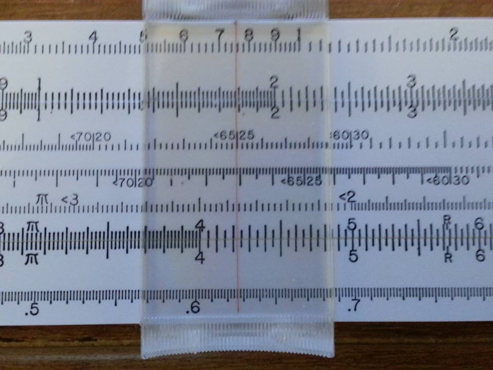
We recall that $\log_{10} 4213 = 3 + \log_{10} 4.213$ . The logarithm on the right-hand side can be estimated by looking at a slide rule. Here’s a picture from my slide rule:

The important parts of this picture are the bottom two rows. Note that the thin red line is lined up between $4.2$ and $4.25$ ; indeed, the red line is about one-third of way from $4.2$ to $4.25$ . On the bottom row, the thin red line is lined up with $0.626$ . So we estimate that $\log_{10} 4213 \approx 3.626$ , so that $\log_{10} \sqrt{4213} \approx \frac{1}{2} (3.626) = 1.813$ .

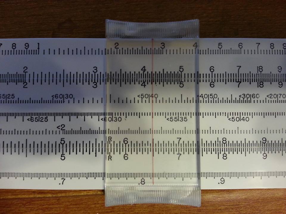
Working the other direction, we must find $10^{1.813} = 10 \times 10^{0.813}$ . We move the thin red line to a different part of the slide rule:

This time, the thin red line is lined up with $0.813$ on the bottom row. On the row above, the red line is lined up almost exactly on $6.5$ , but perhaps a little to the left of $6.5$ . So we estimate that $10^{1.813} \approx 64.9$ or $64.95$ .

The correct answer is $64.907\dots$ .

Not bad for a piece of plastic.

Because taking square roots is so important, many slide rules have lines that simulate a square-root function… without the intermediate step of taking logarithms. Let’s consider again at the above picture, but this time let’s look at the second row from the top. Notice that the thin red line goes between $42$ and $42.5$ on the second line. (FYI, the line repeats itself to the left, so that the user can tell the difference between $42$ and $4.2$ .) Then looking down to the second line from the bottom, we see that the square root is a little less than $65$ , as before.

In addition to square roots, my personal slide rule has lines for cube roots, sines, cosines, and tangents. In the past, more expensive slide rules had additional lines for the values of other mathematical functions.

Square roots and logarithms without a calculator (Part 6)

In Parts 3-5 of this series, I discussed how log tables were used in previous generations to compute logarithms and antilogarithms.

Today’s topic — log tables — not only applies to square roots but also multiplication, division, and raising numbers to any exponent (not just to the $1/2$ power). After showing how log tables were used in the past, I’ll conclude with some thoughts about its effectiveness for teaching students logarithms for the first time.

To begin, let’s again go back to a time before the advent of pocket calculators… say, the 1880s.

Aside from a love of the movies of both Jimmy Stewart and John Wayne, I chose the 1880s on purpose. By the end of that decade, James Buchanan Eads had built a bridge over the Mississippi River and had designed a jetty system that allowed year-round navigation on the Mississippi River. Construction had begun on the Panama Canal. In New York, the Brooklyn Bridge (then the longest suspension bridge in the world) was open for business. And the newly dedicated Statue of Liberty was welcoming American immigrants to Ellis Island.

And these feats of engineering were accomplished without the use of pocket calculators.

Here’s a perfectly respectable way that someone in the 1880s could have computed $\sqrt{4213}$ to reasonably high precision. Let’s write

$x = \sqrt{4213}$ .

Take the base-10 logarithm of both sides.

$\log_{10} x = \log_{10} \sqrt{4213} = \log_{10} (4213)^{1/2} = \displaystyle \frac{1}{2} \log_{10} 4213$ .

Then log tables can be used to compute $\log_{10} 4213$ .

Step 1. In our case, we’re trying to find $\log_{10} 4213$ . We know that $\log_{10} 1000 = 3$ and $\log_{10} 10,000 = 4$ , so the answer must be between $3$ and $4$ . More precisely,

$\log_{10} 4213 = \log_{10} (1000 \times 4.213) = \log_{10} 1000 + \log_{10} 4.213 = 3 + \log_{10} 4.213$ .

To find $\log_{10} 4.213$ , we see from the table that

$\log_{10} 4.21 \approx 0.6243$ and $\log_{10} 4.22 = 0.6253$

So, to estimate $\log_{10} 4.213$ , we will employ linear interpolation. That’s a fancy way of saying “Find the line connecting $(4.21,0.6243)$ and $(4.22,0.6253)$ , and find the point on the line whose $x-$ coordinate is $4.213$ . Finding this line is a straightforward exercise in the point-slope form of a line:

$m = \displaystyle \frac{0.6253-0.6243}{4.22-4.21} = 0.1$

$y - 0.6243 = 0.1 (x - 4.21)$

$y = 0.6243 + 0.1 (4.213-4.21)$

$y = 0.6243 + 0.1(0.003) = 0.6246$

So we estimate $\log_{10} 4.213 \approx 0.6246$ . Thus, so far in the calculation, we have

$\log_{10} \sqrt{4213} \approx \displaystyle \frac{1}{2} (3 + 0.6246) = 1.8123$

Step 2. We then take the antilogarithm of both sides. The term antilogarithm isn’t used much anymore, but the principle is still taught in schools: take $10$ to the power of both the left- and right-hand sides. We obtain

$\sqrt{4213} \approx 10^{1.8123} = 10^{1 + 0.8123} = 10^1 \times 10^{0.8123}$

The first part of the right-hand side is easy: $10^1 = 10$ . For the second-part, we use the log table again, but in reverse. We try to find the numbers that are closest to $0.8123$ in the body of the table. In our case, we find that

$\log_{10} 6.49 = 0.8122$ and $\log_{10} 6.50 = 0.8129$ .

Once again, we use linear interpolation to find the line connecting $(6.49,0.8122)$ and $(6.50,0.8129)$ , except this time the $y-$ coordinate of $0.8123$ is known and the $x-$ coordinate is unknown.

$m = \displaystyle \frac{0.8129-0.8122}{6.50-6.49} = 0.07$

$y - 0.8122 = 0.07 (x - 6.49)$

$0.8123 - 0.8122 = 0.07 (x - 6.49)$

$x = 6.49 + \displaystyle \frac{0.0001}{0.07} = 6.4914\dots$

Since the table is only accurate to four significant digits, we estimate that $10^{0.8123} \approx 6.491$ . Therefore,

$\sqrt{4213} \approx 10^1 \times 10^{0.8123} = 10 \times 6.491 = 64.91$

By way of comparison, the answer is $\sqrt{4213} \approx 64.9076\dots \approx 64.91$ , rounding at the hundredths digit. Not bad, for a generation born before the advent of calculators.

With a little practice, one can do the above calculations with relative ease. Also, many log tables of the past had a column called “proportional parts” that essentially replaced the step of linear interpolation, thus speeding the use of the table considerably.

Log tables can be used for calculations more complex than finding a square root. For example, suppose I need to calculate

$x = \displaystyle \frac{(34.5)^3}{(912)^{2/5}}$

Using the log table, and without using a calculator, I find that

$\log_{10} x = 3 \log_{10} 34.5 - \displaystyle \frac{2}{5} \log_{10} 912$

$\log_{10} x = 3(1.5378) - \displaystyle \frac{2}{5} (2.9600)$

$\log_{10} x = 3.4294$

$x = 10^3 \cdot 10^{0.4294} = 1000 \cdot 2.688 = 2688$

That’s the correct answer to four significant digits. Using a calculator, we find the answer is $2688.186\dots$

Square roots and logarithms without a calculator (Part 5)

One way that square roots can be computed without a calculator is by using log tables. This was a common computational device before pocket scientific calculators were commonly affordable… say, the 1920s.

As many readers may be unfamiliar with this blast from the past, Parts 3 and 4 of this series discussed the mechanics of how to use a log table. In Part 6, I’ll discuss how square roots (and other operations) can be computed with using log tables.

In this post, I consider the modern pedagogical usefulness of log tables, even if logarithms can be computed more easily with scientific calculators.

A personal story: In either 1981 or 1982, my parents bought me my first scientific calculator. It was a thing of beauty… maybe about 25% larger than today’s TI-83s, with an LED screen that tilted upward. When it calculated something like $\log_{10} 4213$ , the screen would go blank for a couple of seconds as it struggled to calculate the answer. I’m surprised that smoke didn’t come out of both sides as it struggled. It must have cost my parents a small fortune, maybe over $1000 after adjusting for inflation. Naturally, being an irresponsible kid in the early 1980s, it didn’t last but a couple of years. (It’s a wonder that my parents didn’t kill me when I broke it.)

So I imagine that requiring all students to use log tables fell out of favor at some point during the 1980s, as technology improved and the prices of scientific calculators became more reasonable.

I regularly teach the use of log tables to senior math majors who aspire to become secondary math teachers. These students who have taken three semesters of calculus, linear algebra, and several courses emphasizing rigorous theorem proving. In other words, they’re no dummies. But when I show this blast from the past to them, they often find the use of a log table to be absolutely mystifying, even though it relies on principles — the laws of logarithms and the point-slope form of a line — that they think they’ve mastered.

So why do really smart students, who after all are math majors about to graduate from college, struggle with mastering log tables, a concept that was expected of 15- and 16-year-olds a generation ago? I personally think that a lot of their struggles come from the fact that they don’t really know logarithms in the way that students of previous generation had to know them in order to survive precalculus. For today’s students, a logarithm is computed so easily that, when my math majors were in high school, they were not expected to really think about its meaning.

For example, it’s no longer automatic for today’s math majors to realize that $\log_{10} 4213$ has to be between $3$ and $4$ someplace. They’ll just punch the numbers in the calculators to get an answer, and the process happens so quickly that the answer loses its meaning.

They know by heart that $\log_{b} xy = \log_{b} x + \log_{b} y$ and that $\log_b b^x = x$ . But it doesn’t reflexively occur to them that these laws can be used to rewrite $\log_{10} 4213$ as $3 + \log_{10} 4.213$ .

When encountering $10^{1.8123}$ , their first thought is to plug into a calculator to get the answer, not to reflect and realize that the answer, whatever it is, has to be between $10$ and $100$ someplace.

Today’s math majors can be taught these approximation principles, of course, but there’s unfortunately no reason to expect that they received the same training with logarithms that students received a generation ago. So none of this discussion should be considered as criticism of today’s math majors; it’s merely an observation about the training that they received as younger students versus the training that previous generations received.

So, do I think that all students today should exclusively learn how to use log tables? Absolutely not.If college students who have received excellent mathematical training can be daunted by log tables, you can imagine how the high school students of generations past must have felt — especially the high school students who were not particularly predisposed to math in the first place.

People like me that made it through the math education system of the 1980s (and before) received great insight into the meaning of logarithms. However, a lot of students back then found these tables as mystifying as today’s college students, and perhaps they did not survive the system because they found the use of the table to be exceedingly complex. In other words, while they were necessary for an era that pre-dated pocket calculators, log tables (and trig tables) were an unfortunate conceptual roadblock to a lot of students who might have had a chance at majoring in a STEM field. By contrast, logarithms are found easily today so that the steps above are not a hindrance to today’s students.

That said, I do argue that there is pedagogical value (as well as historical value) in showing students how to use log tables, even though calculators can accomplish this task much quicker. In other words, I wouldn’t expect students to master the art of performing the above steps to compute logarithms on the homework assignments and exams. But if they can’t perform the above steps, then there’s room for their knowledge of logarithms to grow.

And it will hopefully give today’s students a little more respect for their elders.

Square roots and logarithms without a calculator (Part 4)

I’m in the middle of a series of posts concerning the elementary operation of computing a square root. In Part 3 of this series, I discussed how previous generations computed logarithms without a calculator by using log tables. In this post, I’ll discuss how previous generations computed, using the language of the time, antilogarithms. In Part 5, I’ll discuss my opinions about the pedagogical usefulness of log tables, even if logarithms can be computed more easily with scientific calculators. And in Part 6, I’ll return to square roots — specifically, how log tables can be used to find square roots.

Let’s again go back to a time before the advent of pocket calculators… say, 1943.

The following log tables come from one of my prized possessions: College Mathematics, by Kaj L. Nielsen (Barnes & Noble, New York, 1958).

How to use the table, Part 5. The table can also be used to work backwards and find an antilogarithm. The term antilogarithm isn’t used much anymore, but the principle is still used in teaching students today. Suppose we wish to solve

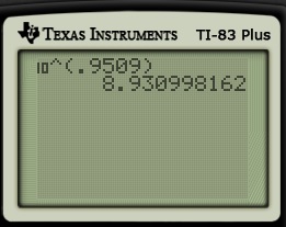
$\log_{10} x = 0.9509$ , or $x = 10^{0.9509}$ .

Looking through the body of the table, we see that $9509$ appears on the row marked $89$ and the column marked $3$ . Therefore, $10^{0.9509} \approx 8.93$. Again, this matches (to three and almost four significant digits) the result of a modern calculator.

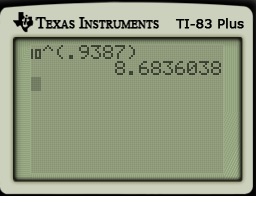
How to use the table, Part 6. Linear interpolation can also be used to find antilogarithms. Suppose we’re trying to evaluate $10^{0.9387}$ , or find the value of $x$ so that $\log_{10} x = 0.9387$. From the table, we can trap $9387$ between

$\log_{10} 8.68 \approx 0.9385$ and $\log_{10} 8.69 \approx 0.9390$

So we again use linear interpolation, except this time the value of $y$ is known and the value of $x$ is unknown:

$m = \displaystyle \frac{0.9390-0.9385}{8.69-8.68} = 0.05$

$y - 0.9385= 0.05 (x - 8.68)$

$0.9387 - 0.9385= 0.05 (x - 8.68)$

$0.0002 = 0.05 (x-8.68)$

$0.004 =x-8.68$

$8.684 =x$

So we estimate $10^{0.9387} \approx 8.684$ This matches the result of a modern calculator to four significant digits:

How to use the table, Part 7.

How to use the table, Part 8.

Note: Sorry, but I’m not sure what happened… when the post came up this morning (August 4), I saw my work in Parts 7 and 8 had disappeared. Maybe one of these days I’ll restore this.

Square roots and logarithms without a calculator (Part 3)

Today’s topic is the use of log tables. I’m guessing that many readers have either forgotten how to use a log table or else were never even taught how to use them. After showing how log tables were used in the past, I’ll conclude with some thoughts about its effectiveness for teaching students logarithms for the first time.

This will be a fairly long post about log tables. In the next post, I’ll discuss how log tables can be used to compute square roots.

To begin, let’s again go back to a time before the advent of pocket calculators… say, 1912.

Before the advent of pocket calculators, most professional scientists and engineers had mathematical tables for keeping the values of logarithms, trigonometric functions, and the like. The following images come from one of my prized possessions: College Mathematics, by Kaj L. Nielsen (Barnes & Noble, New York, 1958). Some saint gave this book to me as a child in the late 1970s; trust me, it was well-worn by the time I actually got to college.

With the advent of cheap pocket calculators, mathematical tables are a relic of the past. The only place that any kind of mathematical table common appears in modern use are in statistics textbooks for providing areas and critical values of the normal distribution, the Student $t$ distribution, and the like.

That said, mathematical tables are not a relic of the remote past. When I was learning logarithms and trigonometric functions at school in the early 1980s — one generation ago — I distinctly remember that my school textbook had these tables in the back of the book.

And it’s my firm opinion that, as an exercise in history, log tables can still be used today to deepen students’ facility with logarithms. In this post and Part 4 of this series, I discuss how the log table can be used to compute logarithms and (using the language of past generations) antilogarithms without a calculator. In Part 5, I’ll discuss my opinions about the pedagogical usefulness of log tables, even if logarithms can be computed more easily nowadays with scientific calculators. In Part 6, I’ll return to square roots — specifically, how log tables can be used to find square roots.

How to use the table, Part 1. How do you read this table? The left-most column shows the ones digit and the tenths digit, while the top row shows the hundredths digit. So, for example, the bottom row shows ten different base-10 logarithms:

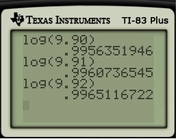
$\log_{10} 9.90 \approx 0.9956, \log_{10} 9.91 \approx 0.9961, \log_{10} 9.92 \approx 0.9965,$

$\log_{10} 9.93 \approx 0.9969, \log_{10} 9.94 \approx 0.9974, \log_{10} 9.95 \approx 0.9978,$

$\log_{10} 9.96 \approx 0.9983, \log_{10} 9.97 \approx 0.9987, \log_{10} 9.98 \approx 0.9991,$

$\log_{10} 9.99 \approx 0.9996$

So, rather than punching numbers into a calculator, the table was used to find these logarithms. You’ll notice that these values match, to four decimal places, the values found on a modern calculator.

How to use the table, Part 2. What if we’re trying to take the logarithm of a number between $1$ and $10$ which has more than two digits after the decimal point, like $\log_{10} 5.1264$ ? From the table, we know that the value has to lie between

$\log_{10} 5.12 \approx 0.7093$ and $\log_{10} 5.13 \approx 0.7101$

So, to estimate $\log_{10} 5.1264$ , we will employ linear interpolation. That’s a fancy way of saying “Find the line connecting $(5.12,0.7093)$ and $(5.13,0.7101)$ , and find the point on the line whose $x-$ coordinate is $5.1264$ . The graph of $y = \log_{10} x$ is not a straight line, of course, but hopefully this linear interpolation will be reasonably close to the correct answer.

Finding this line is a straightforward exercise in the point-slope form of a line:

$m = \displaystyle \frac{0.7101-0.7093}{5.13-5.12} = 0.08$

$y - 0.7093= 0.08 (x - 5.12)$

$y = 0.7093+ 0.08 (5.1264-5.12)$

$y = 0.7093+ 0.08(0.0064) = 0.7093 + 0.000512 = 0.709812$

Remembering that this log table is only good to four significant digits, we estimate $\log_{10} 5.1264 \approx 0.7098$ .

Again, this matches the result of a modern calculator to four decimal places:

How to use the table, Part 3. So far, we’ve discussed taking the logarithms of numbers between $1$ and $10$ and the antilogarithms of numbers between $0$ and $1$ . Let’s now consider what happens if we pick a number outside of these intervals.

To find $\log_{10} 12,345$ , we observe that

$\log_{10}12345 = \log_{10} (10,000 \times 1.2345)$

$\log_{10} 12345 = \log_{10} 10,000 + \log_{10} 1.2345$

$\log_{10} 12345 = 4 + \log_{10} 1.2345$

More intuitively, we know that the answer must lie between $\log_{10} 10,000 = 4$ and $100,000 = 5$ , so the answer must be $4.\hbox{something}$ . The value of $\log_{10} 1.2345$ is the necessary $\hbox{something}$ .

We then find $\log_{10} 1.2345$ by linear interpolation. From the table, we see that

$\log_{10} 1.23 \approx 0.0899$ and $\log_{10} 1.24 \approx 0.0934$

Employing linear interpolation, we find

$m = \displaystyle \frac{0.0934-0.0899}{1.24-1.23} = 0.35$

$y - 0.0899= 0.35 (x - 1.23)$

$y = 0.0899+ 0.35 (1.2345-1.23)$

$y = 0.0899+ 0.35(0.0045) = 0.0899 + 0.001575 = 0.091475$

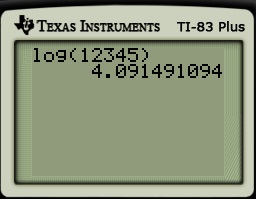
Remembering that this log table is only good to four significant digits, we estimate $\log_{10} 1.2345 \approx 0.0915$ , so that $\log_{10} 12,345 \approx 4.0915$ .

Again, this matches the result of a modern calculator to four decimal places (in this case, five significant digits):

How to use the table, Part 4. Let’s now consider what happens if we pick a positive number less than $1$ . To find $\log_{10} 0.00012345$ , we observe that

$\log_{10}0.00012345 = \log_{10} \left( 1.2345 \times 10^{-4} \right)$

$\log_{10}0.00012345 = \log_{10} 1.2345 + \log_{10} 10^{-4}$

$\log_{10} 0.00012345 = -4 + \log_{10} 1.2345$

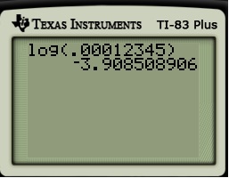
We have already found $\log_{10} 1.2345 \approx 0.0915$ by linear interpolation. We therefore conclude that $\log_{10} 12,345 \approx 0.0915 - 4 = -3.9085$ . Again, this matches the result of a modern calculator to four decimal places (in this case, five significant digits):

So that’s how to compute logarithms without a calculator: we rely on somebody else’s hard work to compute these logarithms (which were found in the back of every precalculus textbook a generation ago), and we make clever use of the laws of logarithms and linear interpolation.

Log tables are of course subject to roundoff errors. (For that matter, so are pocket calculators, but the roundoff happens so deep in the decimal expansion — the 12th or 13th digit — that students hardly ever notice the roundoff error and thus can develop the unfortunate habit of thinking that the result of a calculator is always exactly correct.)

For a two-page table found in a student’s textbook, the results were typically accurate to four significant digits. Professional engineers and scientists, however, needed more accuracy than that, and so they had entire books of tables. A table showing 5 places of accuracy would require about 20 printed pages, while a table showing 6 places of accuracy requires about 200 printed pages. Indeed, if you go to the old and dusty books of any decent university library, you should be able to find these old books of mathematical tables.

In other words, that’s how the Brooklyn Bridge got built in an era before pocket calculators.

At this point you may be asking, “OK, I don’t need to use a calculator to use a log table. But let’s back up a step. How were the values in the log table computed without a calculator?” That’s a perfectly reasonable question, but this post is getting long enough as it is. Perhaps I’ll address this issue in a future post.

Square roots and logarithms without a calculator (Part 2)

I like to show my future secondary teachers a brief history on this topic… partially to deepen their knowledge about what they likely think is a simple concept, but also to give them a little appreciation for their elders. Indeed, when I show this method to today’s college students, they are absolutely mystified that a square root can be extracted by hand, without the aid of a calculator.

To begin, let’s again go back to a time before the advent of pocket calculators… say, ancient Rome. (I personally love using Back to the Future for the pedagogical purpose of simulating time travel, but I already used that in the previous post.)

How did previous generations figure out $\sqrt{4213}$ without a calculator? In the previous post, I introduced a trapping method that directly used the definition of $\sqrt{~~}$ for obtaining one digit at a time. Here’s a second trapping method that’s significantly more efficient. As we’ll see, this second method works because of base-10 arithmetic and a very clever use of Algebra I. My understanding is that this procedure was a standard topic in the mathematical training of children as little as 50 years ago.

Personally, I was taught this method when I was maybe 10 or 11 years old by my math teacher; I don’t doubt that she had to learn to extract square roots by hand when she was a student. Of course, this trapping method fell out of pedagogical favor with the advent of cheap pocket calculators.

I’ll illustrate this method again with $\sqrt{4213}$ . After illustrating the method, I’ll discuss how it works using Algebra I.

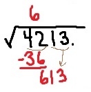
1. To begin, we start from the decimal point and group digits in block of two. (If the number had been $413$ , then the $4$ would have been in a group by itself.) I start with the $42$ . What perfect square is closest to $42$ without going over? Clearly, the answer is $6$ . So, mimicking the algorithm for long division:

We’ll place a $6$ over the $42$ , signifying that the answer is in the $60$ s.
We’ll subtract $36$ from $42$ , for an answer of $6$ .

2. On the next step, we’ll do a couple of things that are different from ordinary long division:

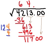
We’ll bring down the next two digits. So we’ll work with $613$ .
We’ll double the number currently on top and place the result to the side. In our case $6 \times 2 = 12$.
We’ll place a small ___ after the $12$ and under the $12$ .
The basic question is: I need $120$ –something times the same something to be as close to $613$ as possible without going over. I like calling this The Price Is Right problem, since so many games on that game show involve guessing a price without going over the actual price. For example…

$121 \times 1 = 121$ : too small

$122 \times 2 = 244$ : too small

$123 \times 3 = 369$ : too small

$124 \times 4 = 496$ : too small

$125 \times 5 = 625$ : too big

Based on the above work, the next digit is $4$ . We place the $4$ over the next block of digits and subtract $124 \times 4 = 496$ from $613$ . So we will work with $613-496 = 117$ on the next step.

3. On the next step, we’ll do a couple of things that are different from ordinary long division:

We’ll bring down the next two digits. On this step, the next two digits are the first two zeroes after the decimal point. So we’ll work with $11,700$ .
We’ll double the number currently on top and place the result to the side. In our case $64 \times 2 = 128$.
We’ll place a small ___ after the $128$ and under the $128$ .
The basic question is: I need $1280$ –something times the same something to be as close to $11,700$ as possible without going over. For example…

$1281 \times 1 = 1281$ : too small

$1282 \times 2 = 2564$ : too small

$1283 \times 3 = 3849$ : too small

$1284 \times 4 = 5136$ : too small

$1285 \times 5 = 6425$ : too small

$1286 \times 6 = 7716$ : too small

$1287 \times 7 = 9009$ : too small

$1288 \times 8 = 10,304$ : too small

$1289 \times 9 = 11,601$ : still too small

Based on the above work, the next digit is $9$ . We place the $9$ over the next block of digits and subtract $1289 \times 9 = 11,601$ from $11,700$ . So we will work with $11,700-11,601 = 99$ on the next step.

Then, to quote The King and I, et cetera, et cetera, et cetera. Each step extracts an extra digit of the square root. With a little practice, one gets better at guessing the correct value of $x$ .

A personal story: when I was a teenager and too cheap to buy a magazine, I would extract square roots to kill time while waiting in the airport for a flight to start boarding. My parents hated missing flights, so I was always at the gate with plenty of time to spare… and I could extract about 20 digits of $\sqrt{2}$ while waiting for the boarding announcement.

So why does this algorithm work? I offer a thought bubble if you’d like to think about before I give the answer.

P.S. In case anyone complains, the people of ancient Rome could not have performed this algorithm since they used Roman numerals and not a base 10 decimal system.

To see why this works, let’s consider the first two steps of finding $\sqrt{4213}$ . Clearly, the answer lies between $60$ and $70$ somewhere (that was Step 1). So the basic problem is to solve for $x$ if

$(60+x)^2 = 4213$ ,

where $x$ is the excess amount over $60$ . Squaring, we obtain

$3600 + 120x + x^2 = 4213$ ,

$120x + x^2 = 613$ ,

$(120+x)x = 613$

Notice that the right-hand side is $4213-3600$ , which was obtained at the start of Step 2. The left-hand side has the form $120$ –something times the same something, which was the key part of completing Step 2. So the value of $x$ that gets $(120+x)x$ as close to $613$ as possible (without going over) will be the next digit in the decimal representation of $\sqrt{4213}$ .

The logic for the remaining digits is similar.

I should mention that third roots, fourth roots, etc. can (in principle) be found using algebra to find excess amounts. However, it’s quite a bit more work for these higher roots. For example, to find the cube root of $4213$ , we immediately see that $10^3 = 1000 < 4213 < 8000 = 20^3$ , so that the answer lies between $10$ and $20$ . To find the excess amount over 10, we need to solve

$(10+x)^3 = 4213$ ,

which reduces to

$(300 + 30x + x^2)x = 3213$ .

So we then try out values of $x$ so that the left-hand side gets as close to $3213$ as possible without going over.

In closing, in honor of this method, here’s a great compilation of clips from The Price Is Right when the contestant guessed a price that was quite close to the actual price without going over.

Square roots and logarithms without a calculator (Part 1)

This post begins a series of posts concerning the elementary operation of computing a square root. This is such an elementary operation because nearly every calculator has a $\sqrt{~~}$ button, and so students today are accustomed to quickly getting an answer without giving much thought to (1) what the answer means or (2) what magic the calculator uses to find square roots.

To begin, let’s go back to a time before the advent of pocket calculators… say, 1955. (When actually teaching this in class, I find the movie clip to be a great and brief way to get students into the mindset of going back in time.)

How did people in 1955 figure out $\sqrt{4213}$ ? After all, plenty of marvelous feats of engineering were made before the advent of calculators. So was this computed back then?

One rudimentary method is simply by trapping the solution. In other words, let’s try guessing the answer to $x^2 = 4213$ and see if we get it right.

1. First, the tens digit.

$60^2 = 3600$ . Too small.
$70^2 = 4900$ . Too big.
Since $3600 < 4213 < 4900$ , the answer has to be somewhere between $60$ and $70$ .

2. Next, the ones digit. Since $4213$ is about halfway between $3600$ and $4900$ , let’s start by guessing $65$ .

$65^2 = 4225$ . Too big, but not much too big. So let’s try $64$ next, as opposed to $62$ or $63$ .
$64^2 = 4096$ . Too small.
So the answer has to be somewhere between $64$ and $65$ .

3. Next, the tenth digit. Since $4213$ is so close to $4225$ , let’s start closer to $65$ than to $64$ .

$64.8^2 = 4199.04$
$64.9^2 = 4212.01$
We already know that $65.0^2 = 4225$
So the answer has to be somewhere between $64.9$ and $65$ .

And we keep repeating this procedure, obtaining one digit at a time. (My next guess, for the hundredths digit, would be $64.91$ or $64.92$ .) Back in 1955, all of the above squaring was done by hand, without a calculator. With enough patience, $\sqrt{4213}$ can be obtained to as many digits as required.

I distinctly remember using this procedure, just for the fun of it, when I was 7 or 8 years old (with the help of calculator, however). This exercise was far more cumbersome that simply hitting the $\sqrt{~~}$ button, but it really developed my number sense as a young child, not to mention internalizing the true meaning of what a square root actually was. Little insights like “let’s start closer to $65$ than to $64$ just don’t come naturally without this kind of trial-and-error practice.

For what it’s worth, the above procedure is the essence of the binary search algorithm (from computer science) or the method of successive bisections (from numerical analysis), with a little human intuition thrown in for good measure.