
Source: http://www.xkcd.com/1153/
See also: https://meangreenmath.com/2013/09/16/formula-for-an-infinite-geometric-series-part-9/
The Mathematical Association of America has an excellent series of 10-minute lectures on various topics in mathematics that are nevertheless accessible to the general public, including gifted elementary school students. The video below is a gentle introduction to knot theory, including computational issues and 3D printing. From the YouTube description:
Laura Taalman, a professor in the Department of Mathematics and Statistics at James Madison University, discusses using technology to explore mathematics.
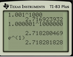
In this series of posts, we have seen that the number 
1. 
 2. We have the limits

These limits form the logical basis for the continuous compound interest formula.
3. We have also shown that 


Therefore, we can let 

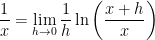
In yesterday’s post, I showed that using the original definition (in terms of an area under a hyperbola) does not lend itself well to numerically approximating
2. The limit 
 3. The best way to compute


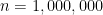
More about approximating
In this series of posts, we have seen that the number
1. 2. We have the limits
These limits form the logical basis for the continuous compound interest formula.
3. We have also shown that
Therefore, we can let
Let’s now consider how the decimal expansion of
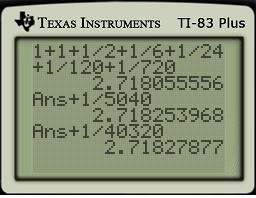
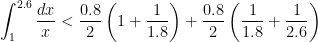
1. Finding ![[1,1.8]](https://s0.wp.com/latex.php?latex=%5B1%2C1.8%5D&bg=ffffff&fg=000000&s=0&c=20201002)
![[1.8,2.6]](https://s0.wp.com/latex.php?latex=%5B1.8%2C2.6%5D&bg=ffffff&fg=000000&s=0&c=20201002)
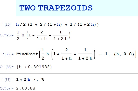
Each trapezoid has a (horizontal) height of 


However, the number 
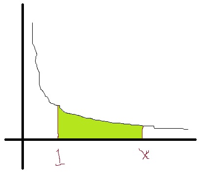
In other words, we know that the area between 
Great, so 


By either guessing and checking — or with the help of Mathematica — it can be determined that this function of 

We can try to better with additional trapezoids. With four trapezoids, we can establish that 
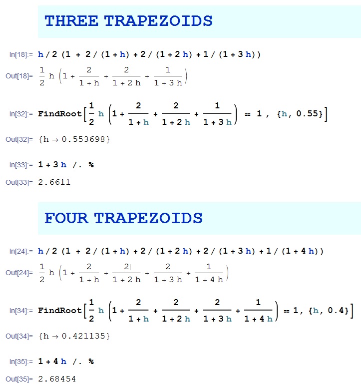
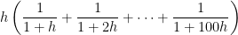
With 100 trapezoids, we can show that 
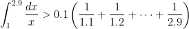
 However, trapezoids can only provide a lower bound on
To obtain an upper bound on 


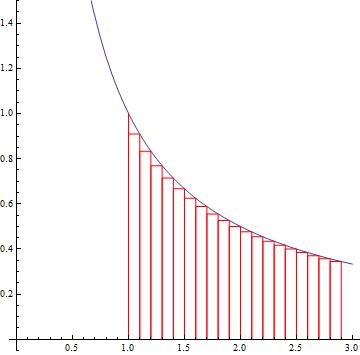 The rectangles all lie below the hyperbola. The width of each one is

In other words, we know that the area between 

Once again, additional rectangles can provide better and better upper bounds on
It then becomes necessary to plug in numbers for
 So with 100 rectangles, we can establish that

Clearly, this is a lot of work for approximating 


In the next post, we’ll explore the other two ways of thinking about the number
In this series of posts, I consider how two different definitions of the number
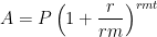
 dollars are invested at interest rate
  for
for  years with continuous compound interest, then the amount of money after years is
  . is defined to be the number so that the area under the curve from to
  is equal to , so that
These two definitions appear to be very, very different. One deals with making money. The other deals with the area under a hyperbola. Amazingly, these two definitions are related to each other. In this series of posts, I’ll discuss the connection between the two.
In yesterday’s post, I proved the following theorem, thus completing a long train of argument that began with the second definition of
Theorem. 
Proof #2. Let’s write the left-hand side as

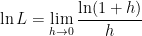
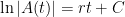
Let’s take the natural logarithm of both sides:
Since 
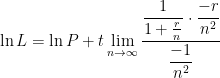
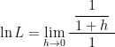
The limit on the right-hand side follows the indeterminate form 

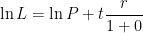
We now solve for the original limit 
In this series of posts, I consider how two different definitions of the number
dollars are invested at interest rate for years with continuous compound interest, then the amount of money after years is . is defined to be the number so that the area under the curve from to is equal to , so that
These two definitions appear to be very, very different. One deals with making money. The other deals with the area under a hyperbola. Amazingly, these two definitions are related to each other. In this series of posts, I’ll discuss the connection between the two.
We begin with the second definition, which is usually considered the true definition of

beginning with this definition of the number
Theorem. 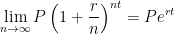
Proof #1.In an earlier post in this series, I showed that
Let’s now replace 


Multiply both sides by
Since
Finally, we multiply both sides by
(A second proof of this theorem, using L’Hopital’s Rule, will be presented in tomorrow’s post.)
This firmly established, at last, the connection between the continuous compound interest formula and the area under the hyperbola. I’ve noted that my students feel a certain sense of accomplishment after reaching this point of the exposition.
In this series of posts, I consider how two different definitions of the number
dollars are invested at interest rate for years with continuous compound interest, then the amount of money after years is . is defined to be the number so that the area under the curve from to is equal to , so that
These two definitions appear to be very, very different. One deals with making money. The other deals with the area under a hyperbola. Amazingly, these two definitions are related to each other. In this series of posts, I’ll discuss the connection between the two.
In yesterday’s post, I proved the following theorem, thus completing a long train of argument that began with the second definition of
Theorem. 
Proof #2. Let’s write the left-hand side as

Let’s take the natural logarithm of both sides:
Since
The right-hand side follows the indeterminate form

Therefore, the original limit is 
In this series of posts, I consider how two different definitions of the number
dollars are invested at interest rate for years with continuous compound interest, then the amount of money after years is . is defined to be the number so that the area under the curve from to is equal to , so that
These two definitions appear to be very, very different. One deals with making money. The other deals with the area under a hyperbola. Amazingly, these two definitions are related to each other. In this series of posts, I’ll discuss the connection between the two.
We begin with the second definition, which is usually considered the true definition of
beginning with this definition of the number
Theorem.
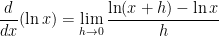
Proof #1. Recall the definition of a derivative

Let’s apply this to the function 
(I’ll note parenthetically that I’ll need the above line for a future post in this series.) At this point, let’s substitute
Let’s now apply the exponential function to both sides:
Since 
Finally, since

(A second proof of this theorem, using L’Hopital’s Rule, will be presented in tomorrow’s post.)
The next theorem establishes, at last, the connection between the continuous compound interest formula and the area under the hyperbola. I’ve noted that my students feel a certain sense of accomplishment after reaching this point of the exposition.
Theorem. 
Proof. Though a little bit of real analysis is necessary to make this rigorous, we can informally see why this has to be true by letting 


In this series of posts, I consider how two different definitions of the number
dollars are invested at interest rate for years with continuous compound interest, then the amount of money after years is . is defined to be the number so that the area under the curve from to is equal to , so that
These two definitions appear to be very, very different. One deals with making money. The other deals with the area under a hyperbola. Amazingly, these two definitions are related to each other. In this series of posts, I’ll discuss the connection between the two.
I should say at the outset that the second definition is usually considered the true definition of
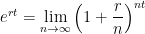
In yesterday’s post, I presented an informal derivation of the continuous compound interest formula 
What does it mean for something to compound continuously? In a nutshell, the rate at which the money increases should be proportional to the amount currently present. In other words, 


for some constant of proportionality
(Technically, a better solution would use an integrating factor [see also MathWorld], but I find that the above derivation is much more convincing to students who are a few semesters removed from a formal course in differential equations.) When presenting this in class, I’ll sometimes lazily write 


To solve for the missing constant 
Replacing 
In this series of posts, I consider how two different definitions of the number
dollars are invested at interest rate for years with continuous compound interest, then the amount of money after years is . is defined to be the number so that the area under the curve from to is equal to , so that
These two definitions appear to be very, very different. One deals with making money. The other deals with the area under a hyperbola. Amazingly, these two definitions are related to each other. In this series of posts, I’ll discuss the connection between the two.
I should say at the outset that the second definition is usually considered the true definition of
At this point in the exposition, I have justified the formula 


We are now in position to give an informal derivation of the continuous compound interest formula. Though this derivation is informal, I have found it to be very convincing for my Precalculus students (as well as to my class of future high school teachers).
The basic idea is to rewrite the discrete compound interest formula so that it contains a term like 

To this end, let 
Inside of the brackets is our familiar friend 


Again, my experience is that college students have no conceptual understanding of this formula or even a memory of seeing it derived once upon a time. They remember is it as coming out of nowhere, as a number in a formula or as a button on a calculator. It really shouldn’t be this way. The above calculation is perhaps a harder sell to high school students that the other calculations that I’ve posted in this series, but I firmly believe that this explanation is within the grasp of good students at the time that they take Algebra II and Precalculus.
Of course, the above derivation is highly informal. For starters, it rests upon the limit

which cannot be formally proven using only the tools of Algebra II and Precalculus. Second, the above computation rests upon the continuity of the function 
So, mathematically speaking, the above argument should not be considered a proper derivation of the continuous compound interest formula. Still, I have found that the above argument to be quite convincing to Algebra II and Precalculus students, appropriate to their current level of mathematical development.


![\ln L = \displaystyle \ln \left[ \lim_{n \to \infty} P \left( 1 + \frac{r}{n} \right)^{nt} \right]](https://s0.wp.com/latex.php?latex=%5Cln+L+%3D+%5Cdisplaystyle+%5Cln+%5Cleft%5B+%5Clim_%7Bn+%5Cto+%5Cinfty%7D+P+%5Cleft%28+1+%2B+%5Cfrac%7Br%7D%7Bn%7D+%5Cright%29%5E%7Bnt%7D+%5Cright%5D&bg=ffffff&fg=000000&s=0&c=20201002)
![\ln L = \displaystyle \lim_{n \to \infty} \ln \left[ P \left( 1 + \frac{r}{n} \right)^{nt} \right]](https://s0.wp.com/latex.php?latex=%5Cln+L+%3D+%5Cdisplaystyle+%5Clim_%7Bn+%5Cto+%5Cinfty%7D+%5Cln+%5Cleft%5B+P+%5Cleft%28+1+%2B+%5Cfrac%7Br%7D%7Bn%7D+%5Cright%29%5E%7Bnt%7D+%5Cright%5D&bg=ffffff&fg=000000&s=0&c=20201002)
![\ln L = \displaystyle \lim_{n \to \infty} \left[ \ln P + \ln \left( 1 + \frac{r}{n} \right)^{nt} \right]](https://s0.wp.com/latex.php?latex=%5Cln+L+%3D+%5Cdisplaystyle+%5Clim_%7Bn+%5Cto+%5Cinfty%7D+%5Cleft%5B+%5Cln+P+%2B+%5Cln+%5Cleft%28+1+%2B+%5Cfrac%7Br%7D%7Bn%7D+%5Cright%29%5E%7Bnt%7D+%5Cright%5D&bg=ffffff&fg=000000&s=0&c=20201002)
![\ln L = \displaystyle \lim_{n \to \infty} \left[ \ln P + nt \ln \left( 1 + \frac{r}{n} \right)\right]](https://s0.wp.com/latex.php?latex=%5Cln+L+%3D+%5Cdisplaystyle+%5Clim_%7Bn+%5Cto+%5Cinfty%7D+%5Cleft%5B+%5Cln+P+%2B+nt+%5Cln+%5Cleft%28+1+%2B+%5Cfrac%7Br%7D%7Bn%7D+%5Cright%29%5Cright%5D&bg=ffffff&fg=000000&s=0&c=20201002)


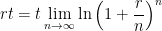

![rt = \displaystyle \lim_{n \to \infty} \ln \left[ \left(1 + \frac{r}{n} \right)^{n} \right]^t](https://s0.wp.com/latex.php?latex=rt+%3D+%5Cdisplaystyle+%5Clim_%7Bn+%5Cto+%5Cinfty%7D+%5Cln+%5Cleft%5B+%5Cleft%281+%2B+%5Cfrac%7Br%7D%7Bn%7D+%5Cright%29%5E%7Bn%7D+%5Cright%5D%5Et&bg=ffffff&fg=000000&s=0&c=20201002)
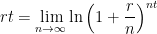
![rt = \displaystyle \ln \left[ \lim_{n \to \infty} \left(1 + \frac{r}{n} \right)^{nt} \right]](https://s0.wp.com/latex.php?latex=rt+%3D+%5Cdisplaystyle+%5Cln+%5Cleft%5B+%5Clim_%7Bn+%5Cto+%5Cinfty%7D+%5Cleft%281+%2B+%5Cfrac%7Br%7D%7Bn%7D+%5Cright%29%5E%7Bnt%7D+%5Cright%5D&bg=ffffff&fg=000000&s=0&c=20201002)

![\ln L = \displaystyle \ln \left[ \lim_{h \to 0} \left( 1 + h \right)^{1/h} \right]](https://s0.wp.com/latex.php?latex=%5Cln+L+%3D+%5Cdisplaystyle+%5Cln+%5Cleft%5B+%5Clim_%7Bh+%5Cto+0%7D+%5Cleft%28+1+%2B+h+%5Cright%29%5E%7B1%2Fh%7D+%5Cright%5D&bg=ffffff&fg=000000&s=0&c=20201002)


![e^1 = \exp \left[ \displaystyle \lim_{h \to 0} \ln (1 + h)^{1/h} \right]](https://s0.wp.com/latex.php?latex=e%5E1+%3D+%5Cexp+%5Cleft%5B+%5Cdisplaystyle+%5Clim_%7Bh+%5Cto+0%7D+%5Cln+%281+%2B+h%29%5E%7B1%2Fh%7D+%5Cright%5D&bg=ffffff&fg=000000&s=0&c=20201002)
![e = \displaystyle \lim_{h \to 0} \exp \left[ \ln (1 + h)^{1/h} \right]](https://s0.wp.com/latex.php?latex=e+%3D+%5Cdisplaystyle+%5Clim_%7Bh+%5Cto+0%7D+%5Cexp+%5Cleft%5B+%5Cln+%281+%2B+h%29%5E%7B1%2Fh%7D+%5Cright%5D&bg=ffffff&fg=000000&s=0&c=20201002)


![A = P\displaystyle \left[ \left( 1 + \frac{1}{m} \right)^m \right]^{rt}](https://s0.wp.com/latex.php?latex=A+%3D+P%5Cdisplaystyle+%5Cleft%5B+%5Cleft%28+1+%2B+%5Cfrac%7B1%7D%7Bm%7D+%5Cright%29%5Em+%5Cright%5D%5E%7Brt%7D&bg=ffffff&fg=000000&s=0&c=20201002)

