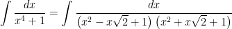
This antiderivative has arguable the highest ratio of “really hard to compute” to “really easy to write”:

$\displaystyle \int \frac{1}{x^4 + 1} dx$

So far, I’ve shown that the denominator can be factored over the real numbers:

$\displaystyle \int \frac{dx}{x^4 + 1} = \displaystyle \int \frac{dx}{\left(x^2 - x \sqrt{2} + 1 \right) \left(x^2 + x \sqrt{2} + 1\right)}$

$= \displaystyle \int \frac{ -\displaystyle \frac{\sqrt{2}}{4} x + \frac{1}{2}}{ x^2 - x \sqrt{2} + 1 } dx + \int \frac{ \displaystyle \frac{\sqrt{2}}{4} x + \frac{1}{2}}{ x^2 + x \sqrt{2} + 1 } dx$

after finding the partial fractions decomposition.

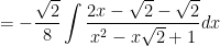
Let me start with the first of the two integrals. It’d be nice to use the substitution $u = x^2 - x \sqrt{2} + 1$ . However, $du = (2x - \sqrt{2}) dx$ , and so this substitution can’t be used cleanly. So, let me force the numerator to have this form, at least in part:

$= \displaystyle \int \frac{ -\displaystyle \frac{\sqrt{2}}{4} x + \frac{1}{2}}{ x^2 - x \sqrt{2} + 1 } dx = \displaystyle -\frac{\sqrt{2}}{4} \int \frac{ x - \sqrt{2}}{ x^2 - x \sqrt{2} + 1 } dx$

$= \displaystyle -\frac{\sqrt{2}}{8} \int \frac{2x - 2\sqrt{2}}{ x^2 - x \sqrt{2} + 1 } dx$

$= \displaystyle -\frac{\sqrt{2}}{8} \int \frac{ 2x - \sqrt{2} - \sqrt{2} }{ x^2 - x \sqrt{2} + 1 } dx$

$= \displaystyle -\frac{\sqrt{2}}{8} \int \frac{ 2x - \sqrt{2} }{ x^2 - x \sqrt{2} + 1 } dx + \frac{1}{4} \int \frac{ dx }{ x^2 - x \sqrt{2} + 1 }$

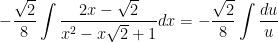
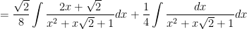
The substitution can now be applied to the first integral:

$\displaystyle -\frac{\sqrt{2}}{8} \int \frac{2x - \sqrt{2} }{ x^2 - x \sqrt{2} + 1 } dx = \displaystyle -\frac{\sqrt{2}}{8} \int \frac{du}{u}$

$= \displaystyle -\frac{\sqrt{2}}{8} \ln |u| + C$

$= \displaystyle -\frac{\sqrt{2}}{8} \ln |x^2 - x\sqrt{2} + 1| + C$

$= \displaystyle -\frac{\sqrt{2}}{8} \ln (x^2 - x\sqrt{2} + 1) + C$ .

On the last line, I was able to remove the absolute value signs because $x^2 - x \sqrt{2} + 1$ is an irreducible quadratic and hence is never equal to zero for any real number $x$ .

Similarly, I’ll try to apply the substitution $v = x^2 + x \sqrt{2} + 1$ to the second integral:

$= \displaystyle \int \frac{ \displaystyle \frac{\sqrt{2}}{4} x + \frac{1}{2}}{ x^2 + x \sqrt{2} + 1 } dx = \displaystyle \frac{\sqrt{2}}{4} \int \frac{ x + \sqrt{2}}{ x^2 + x \sqrt{2} + 1 } dx$

$= \displaystyle \frac{\sqrt{2}}{8} \int \frac{ 2x + 2\sqrt{2}}{ x^2 + x \sqrt{2} + 1 } dx$

$= \displaystyle \frac{\sqrt{2}}{8} \int \frac{2x + \sqrt{2} + \sqrt{2} }{ x^2 + x \sqrt{2} + 1 } dx$

$= \displaystyle \frac{\sqrt{2}}{8} \int \frac{2x + \sqrt{2} }{ x^2 + x \sqrt{2} + 1 } dx + \frac{1}{4} \int \frac{ dx }{ x^2 + x \sqrt{2} + 1 } dx$

The substitution can now be applied to the first integral:

$\displaystyle \frac{\sqrt{2}}{8} \int \frac{2x + \sqrt{2} }{ x^2 + x \sqrt{2} + 1 } dx = \displaystyle \frac{\sqrt{2}}{8} \int \frac{dv}{v}$

$= \displaystyle \frac{\sqrt{2}}{8} \ln |v| + C$

$= \displaystyle \frac{\sqrt{2}}{8} \ln |x^2 + x\sqrt{2} + 1| + C$

$= \displaystyle \frac{\sqrt{2}}{8} \ln (x^2 + x\sqrt{2} + 1) + C$ .

So, thus far, I have shown that

$\displaystyle \int \frac{dx}{x^4 + 1} = \displaystyle -\frac{\sqrt{2}}{8} \ln (x^2 - x\sqrt{2} + 1) + \frac{\sqrt{2}}{8} \ln (x^2 + x\sqrt{2} + 1)$

$\displaystyle + \frac{1}{4} \int \frac{ dx }{ x^2 - x \sqrt{2} + 1 } + \frac{1}{4} \int \frac{ dx }{ x^2 + x \sqrt{2} + 1 } dx$

$= \displaystyle \frac{\sqrt{2}}{8} \ln \left( \frac{x^2 + x\sqrt{2} + 1}{x^2 - x\sqrt{2} + 1} \right) + \frac{1}{4} \int \frac{ dx }{ x^2 - x \sqrt{2} + 1 } + \frac{1}{4} \int \frac{ dx }{ x^2 + x \sqrt{2} + 1 } dx$

I’ll consider the evaluation of the remaining two integrals in tomorrow’s post.

Proving theorems and special cases (Part 13): Uniqueness of logarithms

In a recent class with my future secondary math teachers, we had a fascinating discussion concerning how a teacher should respond to the following question from a student:

Is it ever possible to prove a statement or theorem by proving a special case of the statement or theorem?

Usually, the answer is no. In this series of posts, we’ve seen that a conjecture could be true for the first 40 cases or even the first $10^{316}$ cases yet not always be true. We’ve also explored the computational evidence for various unsolved problems in mathematics, noting that even this very strong computational evidence, by itself, does not provide a proof for all possible cases.

However, there are plenty of examples in mathematics where it is possible to prove a theorem by first proving a special case of the theorem. For the remainder of this series, I’d like to list, in no particular order, some common theorems used in secondary mathematics which are typically proved by first proving a special case.

The next theorem is needed in calculus to show that $\ln x = \displaystyle \int_1^x \frac{dt}{t}$ .

4. Theorem. Let $a \in \mathbb{R}^+ \setminus \{1\}$ . Suppose that $f: \mathbb{R}^+ \rightarrow \mathbb{R}$ has the following four properties:

$f(1) = 0$
$f(a) = 1$
$f(xy) = f(x) + f(y)$ for all $x, y \in \mathbb{R}^+$
$f$ is continuous

Then $f(x) = \log_a x$ for all $x \in \mathbb{R}^+$ .

In other blog posts, I went through the full proof of this theorem, which is divided — actually, scaffolded — into cases:

Case 1. $f(x) = \log_a x$ if $x$ is a positive integer.

Case 2. $f(x) = \log_a x$ if $x$ is a positive rational number.

Case 3. $f(x) = \log_a x$ if $x$ is a negative rational number.

Case 4. $f(x) = \log_a x$ if $x$ is a real number.

Clearly, Case 1 is a subset of Case 2, and Case 3 is a subset of Case 4. Once again, a special case of a theorem is used to prove the full theorem.

Lessons from teaching gifted elementary school students: Index

I’m doing something that I should have done a long time ago: collect past series of posts into a single, easy-to-reference post. The following posts formed my series on various lessons I’ve learned while trying to answer the questions posed by gifted elementary school students.

Part 1: A surprising pattern in some consecutive perfect squares.

Part 2: Calculating 2 to a very large exponent.

Part 3a: Calculating 2 to an even larger exponent.

Part 3b: An analysis of just how large this number actually is.

Part 4a: The chance of winning at BINGO in only four turns.

Part 4b: Pedagogical thoughts on one step of the calculation.

Part 4c: A complicated follow-up question.

Engaging students: Solving logarithmic equations

In my capstone class for future secondary math teachers, I ask my students to come up with ideas for engaging their students with different topics in the secondary mathematics curriculum. In other words, the point of the assignment was not to devise a full-blown lesson plan on this topic. Instead, I asked my students to think about three different ways of getting their students interested in the topic in the first place.

I plan to share some of the best of these ideas on this blog (after asking my students’ permission, of course).

This student submission again comes from my former student Kelley Nguyen. Her topic: how to engage Algebra II or Precalculus students when solving logarithmic equations.

How could you as a teacher create an activity or project that involves your topic? (Flashcard/Match Game)

Because the rules behind logarithms can be mastered with practice, I believe an activity would help the students understand and master the concept. For an activity, I would create a matching game. It will include multiple cards that have logarithmic equations, as well as a match card with its solution or rewritten equation. For example:

The students would be in groups of 2-4 players. The deck of cards will be well-shuffled and laid out face down. Player 1 will turn over two cards and determine if they’re a match. If they’re a matching pair, the student will keep the two cards. If they are not, the player will turn the cards face down again and now it’s Player 2’s turn. If the Player 1 found a match, he/she will go again, following their first attempt. The other players should be observing and checking each other’s pairs to ensure that they are correct matches. They can also help each other in the process, i.e. coaching.

Another activity can also be done with logarithmic equation and solution cards. In this activity, there are 2-4 players in each group. Each player will receive five cards from the deck and the rest of the deck will be placed in the middle of the players in one stack and face down. The players are able to look at their cards and think of the solutions to them. Player 1 will turn the top card in the deck face up. If Player 1 has a matching card, he/she will take the card and start a stack of his/her matching pairs then draw a card from the deck. [Note: players will have five cards at all times.] If Player 1 does not have a match, each player will take a turn. If there is no match, Player 2 will then flip the second card and repeat the process. When all cards in the deck have been flipped over, turn the entire deck face down again and continue. The game will go on until all cards are match up. Whoever has the most matched pairs wins the game.

How can this topic be used in your students’ future courses in mathematics or science?

Logarithms are used frequently in chemistry when learning about acidity. In particular, the following equation describes a derivation of pH as the measure of acidity, as well as estimating the pH of a buffer solution and finding pH at equilibrium in acid-base reactions.

$pH = pK_\alpha + \log_{10} \left( \displaystyle \frac{ [A^-]}{[HA]} \right)$

There is also a time when logarithms are used in physics when working with the Beer-Lambert Law. The intensity of a light I_o passing through a length of size l of a solution of concentration c is given as follows:

$\log (I_0 ll) = \epsilon c l$ ,

where $\epsilon$ is the absorption coefficient.

Another way logarithms are utilized is in science courses when students are to make predictions on the spread of disease in the world. This issue is greatly seen as the population grows dramatically, and using a logarithmic approach will allow the student to make a reasonable guesstimate.

Because students are introduced to logarithms at the end of Algebra II, they will work with them a lot in pre-calculus, as well as into calculus when dealing with trigonometric equations where there is a variable in the base and in the exponent.

How can technology be used to effectively engage students with this topic? (graphing calculator)

Although I think it’s easier to punch logarithmic equations into a calculator to get an answer, I still think that the students should conceptually learn why we come up with the answer. So, before allowing students to use calculators, make sure they know how we came up with the solutions. Once the students have mastered that concept, let them explore with their graphing calculators.

First, have the students put in the basic log function in Y₁, then give them a log function with a transformation, whether it be a vertical shift, horizontal shift, or expansion, and store it into Y₂. Ask the students to describe what they see.

Another way to utilize calculators with this topic is showing that the properties of logs are true, such as the addition rules of logarithmic equations being the log of the product of the arguments. You can also show the students how to change the base of a logarithmic equation on their calculators, since the standard log key is programmed at log₁₀. That can be found when you click MATH and choice A in the first drop-down list.

References

(Unknown). “Log Bases and Log equations”. Lake Tahoe Community College Math Department. Retrieved 7 Nov 2014 from http://www.ltcconline.net/greenl/courses/154/logexp/explogeq.htm
(Unknown). “Solving Logarithmic Equations and Inequalities”. Glencoe Graphing Technology Lab. Retrieved 7 Nov 2014 from http://glencoe.com/sites/common_assets/mathematics/alg2_2010/other_cal_keystrokes/Casio/Casio_523_524_C08_L06B_888482.pdf
Yates, Paul. (May 2009). “Logarithms”. Royal Society of Chemistry. Retrieved 7 Nov 2014 from http://www.rsc.org/education/eic/issues/2009May/logarithms-maths-chemistry.asp

Different definitions of logarithm: Index

I’m doing something that I should have done a long time ago: collect past series of posts into a single, easy-to-reference post. The following posts formed my series on how the different definitions of logarithm are in fact equivalent.

Part 1: Introduction to the two definitions: an antiderivative and an inverse function.

Part 2: The main theorem: four statements only satisfied by the logarithmic function.

Part 3: Case 1 of the proof: positive integers.

Part 4: Case 2 of the proof: positive rational numbers.

Part 5: Case 3 of the proof: negative rational numbers.

Part 6: Case 4 of the proof: irrational numbers.

Part 7: Showing that the function $f(x) = \displaystyle \int_1^x \frac{dt}{t}$ satisfies the four statements.

Part 8: Computation of standard integrals and derivatives involving logarithmic and exponential functions.

The number of digits in n! (Part 4)

When I was in school, I stared at this graph for weeks, if not months, trying to figure out an equation for the number of digits in $n!$ . And I never could figure it out. However, even though I was not able to figure this out for myself, there is a very good approximation using Stirling’s approximation. The next integer after $\log_{10} n!$ gives the number of digits in $n!$ , and

$\log_{10} n! \approx \displaystyle \frac{\left(n + \displaystyle \frac{1}{2} \right) \ln n - n + \displaystyle \frac{1}{2} \ln (2\pi)}{\ln 10}$

The graph below shows just how accurate this approximation really is. The solid curve is the approximation; the dots are the values of $\log_{10} n!$ . Not bad at all… the error in the curve is smaller than the size of the dots.

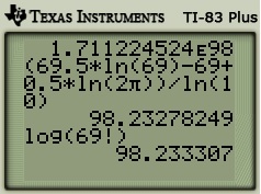
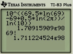
The following output from a calculator shows just how close the approximation to $log_{10} 69!$ is to the real answer. There are also additional terms to Stirling’s series that would get even closer answers.

As I mentioned earlier in this series, I’m still mildly annoyed with my adolescent self that I wasn’t able to figure this out for myself… especially given the months that I spent staring at this problem trying to figure out the answer.

First, I’m annoyed that I didn’t think to investigate $\log_{10} n!$ . I had ample experience using log tables (after all, this was the 1980s, before scientific calculators were in the mainstream) and I should have known this.

Second, I’m annoyed that I didn’t have at the tips of my fingers the change of base formula

$\log_{10} n! = \displaystyle \frac{\ln n!}{\ln 10}$

Third, I’m annoyed that, even though I knew calculus pretty well, I wasn’t able to get at least the first couple of terms of Stirling’s series on my own even though the derivation was entirely in my grasp. To begin,

$\ln n! = \ln (1 \cdot 2 \cdot 3 \dots \cdot n) = \ln 1 + \ln 2 + \ln 3 + \dots + \ln n$

For example, if $n = 10$ , then $\ln 10!$ would be the areas of the 9 rectangles shown below (since $\ln 1 = 0$):

The areas of these nine rectangles is closely approximated by the area under the curve $y = \ln x$ between $x =1\frac{1}{2}$ and $x = 10\frac{1}{2}$ . (Indeed, I chose a Riemann sum with midpoints so that the approximation between the Riemann sum and the integral would be very close.)

In general, for $n!$ instead of $10!$ , we have

$\ln n! \approx \displaystyle \int_{3/2}^{n+1/2} \ln x \, dx$

This is a standard integral that can be obtained via integration by parts:

$\ln n! \approx \bigg[ \displaystyle x \ln x - x \bigg]_{3/2}^{n+1/2}$

$\ln n! \approx \left[ \left(n + \displaystyle \frac{1}{2} \right) \ln \left(n + \displaystyle \frac{1}{2} \right) - \left(n + \displaystyle \frac{1}{2} \right) \right] - \left[ \displaystyle \frac{3}{2} \ln \frac{3}{2} - \frac{3}{2} \right]$

$\ln n! \approx \left(n + \displaystyle \frac{1}{2} \right) \ln \left(n + \displaystyle \frac{1}{2} \right) - n - \displaystyle \frac{3}{2} \ln \frac{3}{2} + 1$

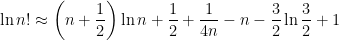
We can see that this is already taking the form of Stirling’s approximation, given above. Indeed, this is surprisingly close. Let’s use the Taylor approximation $\ln(1+x) \approx x$ for $x \approx 0$ :

$\ln n! \approx \left(n + \displaystyle \frac{1}{2} \right) \ln \left(n \left[1 + \displaystyle \frac{1}{2n}\right] \right) - n - \displaystyle \frac{3}{2} \ln \frac{3}{2} + 1$

$\ln n! \approx \left(n + \displaystyle \frac{1}{2} \right) \left[\ln n + \ln \left(1 + \displaystyle \frac{1}{2n} \right) \right] - n - \displaystyle \frac{3}{2} \ln \frac{3}{2} + 1$

$\ln n! \approx \left(n + \displaystyle \frac{1}{2} \right) \left[\ln n + \displaystyle \frac{1}{2n} \right] - n - \displaystyle \frac{3}{2} \ln \frac{3}{2} + 1$

$\ln n! \approx \left(n + \displaystyle \frac{1}{2} \right) \ln n + \left(n + \displaystyle \frac{1}{2} \right) \displaystyle \frac{1}{2n} - n - \displaystyle \frac{3}{2} \ln \frac{3}{2} + 1$

$\ln n! \approx \left(n + \displaystyle \frac{1}{2} \right) \ln n +\displaystyle \frac{1}{2} + \frac{1}{4n} - n - \displaystyle \frac{3}{2} \ln \frac{3}{2} + 1$

$\ln n! \approx \left(n + \displaystyle \frac{1}{2} \right) \ln n - n + \left(\displaystyle \frac{3}{2} - \displaystyle \frac{3}{2} \ln \frac{3}{2} \right) + \displaystyle \frac{1}{4n}$

By way of comparison, the first few terms of the Stirling series for $\ln n!$ are

$\ln n! \approx \left(n + \displaystyle \frac{1}{2} \right) \ln n - n + \displaystyle \frac{1}{2} \ln (2\pi) + \displaystyle \frac{1}{12n}$

We see that the above argument, starting with an elementary Riemann sum, provides the first two significant terms in this series. Also, while the third term is incorrect, it’s closer to the correct third term that we have any right to expect:

$\displaystyle \frac{3}{2} - \displaystyle \frac{3}{2} \ln \frac{3}{2} \approx 0.8918\dots$

$\displaystyle \frac{1}{2} \ln (2\pi) \approx 0.9189\dots$

The correct third term of $\displaystyle \frac{1}{2} \ln(2\pi)$ can also be found using elementary calculus, though the argument is much more sophisticated that the one above. See the MathWorld website for details.

The number of digits in n! (Part 3)

The following graph shows the number of digits in $n!$ as a function of $n$ .

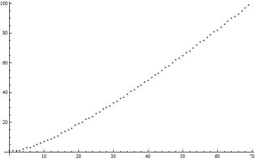
When I was in school, I stared at this graph for weeks, if not months, trying to figure out an equation that would fit these points. And I never could figure it out.

When I took calculus in college, I distinctly remember getting up the nerve to ask my professor, the great L.Craig Evans (now at UC Berkeley), if he knew how to solve this problem. To my great consternation, he immediately wrote down what I now realize to be the right answer, using Stirling’s approximation:

$\ln n! \approx \left(n + \displaystyle \frac{1}{2} \right) \ln n - n + \frac{1}{2} \ln (2\pi)$

While I now know that this was the way to go about solving this problem, I didn’t appreciate how this formula could help me at the time. I only saw the $n!$ on the left-hand side and did not see the immediate connection between this formula and the number of digits in $n!$ .

But now I know better.

For starters, the number of base-10 digits in a number $n$ is always the next integer greater that $\log_{10} n$ . For example, $\log_{10} 2000 \approx 3.301$, and the next integer larger than $3.301$ is 4. Unsurprisingly, the number $2000$ has 4 digits.

Second, the change of base formula for logarithms gives

$\log_{10} n! = \displaystyle \frac{\ln n!}{\ln 10}$

Therefore, the number of digits in $n!$ will be about

$\displaystyle \frac{\left(n + \displaystyle \frac{1}{2} \right) \ln n - n + \frac{1}{2} \ln (2\pi)}{\ln 10}$

The graph below shows just how accurate this approximation really is. The solid curve is the approximation; the dots are the values of $\log_{10} n!$ . (In other words, this series of dots are only slightly different than the dots above, which have integers as coordinates.) Not bad at all… the error in the approximation is smaller than the size of the dots in this picture.

The number of digits in n! (Part 2)

The following graph shows the number of digits in $n!$ as a function of $n$ .

When I was in school, I stared at this graph for weeks, if not months, trying to figure out an equation that would fit these points. And I never could figure it out.

In retrospect, my biggest mistake was thinking that the formula had to be something like $y = a x^m$ , where the exponent $m$ was a little larger than 1. After all, the graph is clearly not a straight line, but it’s also not as curved as a parabola.

What I didn’t know then, but know now, is that there’s a really easy way to determine to determine if a data set exhibits power-law behavior. If $y = a x^m$ , then

$\ln y = \ln a + m \ln x$ .

If we make the substitutions $Y = \ln Y$ , $B = \ln a$ , and $X = \ln x$ , then this equation becomes

$Y = m X + B$

In other words, if the data exhibits power-law behavior, then the log-transformed data would look very much like a straight line. Well, here’s the graph of $(X,Y)$ after applying the transformation:

Ignoring the first couple of pots, the dots show an ever-so-slight concave down pattern, but not enough that would have discouraged me from blindly trying a pattern like $y = a x^m$ . However, because these points do not lie on a straight line and exhibit heteroscedastic behavior, my adolescent self was doomed to failure.

Calculators and Complex Numbers: Index

I’m using the Twelve Days of Christmas (and perhaps a few extra days besides) to do something that I should have done a long time ago: collect past series of posts into a single, easy-to-reference post. The following posts formed my series on how the trigonometric form of complex numbers, DeMoivre’s Theorem, and extending the definitions of exponentiation and logarithm to complex numbers.

Part 1: Introduction: using a calculator to find surprising answers for $\ln(-5)$ and $\sqrt[3]{-8}$ . See the video below.

Part 2: The trigonometric form of complex numbers.

Part 3: Proving the theorem

$\left[ r_1 (\cos \theta_1 + i \sin \theta_1) \right] \cdot \left[ r_2 (\cos \theta_2 + i \sin \theta_2) \right] = r_1 r_2 (\cos [\theta_1+\theta_2] + i \sin [\theta_1+\theta_2])$

Part 4: Proving the theorem

$\displaystyle \frac{ r_1 (\cos \theta_1 + i \sin \theta_1) }{ r_2 (\cos \theta_2 + i \sin \theta_2) } = \displaystyle \frac{r_1}{r_2} (\cos [\theta_1-\theta_2] + i \sin [\theta_1-\theta_2])$