In this series of posts, I’d like to describe what I tell my students on the very first day of Calculus I. On this first day, I try to set the table for the topics that will be discussed throughout the semester. I should emphasize that I don’t hold students immediately responsible for the content of this lecture. Instead, this introduction, which usually takes 30-45 minutes, depending on the questions I get, is meant to help my students see the forest for all of the trees. For example, when we start discussing somewhat dry topics like the definition of a continuous function and the Mean Value Theorem, I can always refer back to this initial lecture for why these concepts are ultimately important.
I’ve told students that the topics in Calculus I build upon each other (unlike the topics of Precalculus), but that there are going to be two themes that run throughout the course:
- Approximating curved things by straight things, and
- Passing to limits
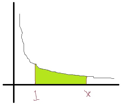
We are now trying to answer the following problem.
Problem #2. Find the area under the parabola  between
  and
and  .
.
Using five rectangles with right endpoints, we find the approximate answer of  . With ten rectangles, the approximation is
  . With one hundred rectangles (and Microsoft Excel), the approximation is
  . This last expression was found by evaluating
![0.01[ (0.01)^2 + (0.02)^2 + \dots + (0.99)^2 + 1^2]](https://s0.wp.com/latex.php?latex=0.01%5B+%280.01%29%5E2+%2B+%280.02%29%5E2+%2B+%5Cdots+%2B+%280.99%29%5E2+%2B+1%5E2%5D&bg=ffffff&fg=000000&s=0&c=20201002)
At this juncture, what I’ll do depends on my students’ background. For many years, I had the same group of students for both Precalculus and Calculus I, and so I knew full well that they had seen the formula for  . And so I’d feel comfortable showing my students the contents of this post. However, if I didn’t know for sure that my students had at least seen this formula, I probably would just ask them to guess the limiting answer without doing any of the algebra to follow.
Assuming students have the necessary prerequisite knowledge, I’ll ask, “What happens if we have  rectangles?” Without much difficulty, they’ll see that the rectangles have a common width of
  . The heights of the rectangles take a little more work to determine. I’ll usually work left to right. The left-most rectangle has right-most
  coordinate of , and so the height of the leftmost rectangle is
  . The next rectangle has a height of
  , and so we must evaluate
![\displaystyle \frac{1}{n} \left[ \frac{1^2}{n^2} + \frac{2^2}{n^2} + \dots + \frac{n^2}{n^2} \right]](https://s0.wp.com/latex.php?latex=%5Cdisplaystyle+%5Cfrac%7B1%7D%7Bn%7D+%5Cleft%5B+%5Cfrac%7B1%5E2%7D%7Bn%5E2%7D+%2B+%5Cfrac%7B2%5E2%7D%7Bn%5E2%7D+%2B+%5Cdots+%2B+%5Cfrac%7Bn%5E2%7D%7Bn%5E2%7D+%5Cright%5D&bg=ffffff&fg=000000&s=0&c=20201002) , or
, or
![\displaystyle \frac{1}{n^3} \left[ 1^2 + 2^2 + \dots + n^2 \right]](https://s0.wp.com/latex.php?latex=%5Cdisplaystyle+%5Cfrac%7B1%7D%7Bn%5E3%7D+%5Cleft%5B+1%5E2+%2B+2%5E2+%2B+%5Cdots+%2B+n%5E2+%5Cright%5D&bg=ffffff&fg=000000&s=0&c=20201002)
I then ask my class, what’s the formula for this sum? Invariably, they’ve forgotten the formula in the five or six weeks between the end of Precalculus and the start of Calculus I, and I’ll tease them about this a bit. Eventually, I’ll give them the answer (or someone volunteers an answer that’s either correct or partially correct):
 , or
, or  .
.
I’ll then directly verify that our previous numerical work matches this expression by plugging in  ,
,  , and
, and  .
.
I then ask, “What limit do we need to take this time?” Occasionally, I’ll get the incorrect answer of sending to zero, as students sometimes get mixed up thinking about the width of the rectangles instead of the number of rectangles. Eventually, the class will agree that we should send to plus infinity. Fortunately, the answer  is an example of a rational function, and so the horizontal asymptote can be immediately determined by dividing the leading coefficients of the numerator and denominator (since both have degree 2). We conclude that the limit is
  , and so that’s the area under the parabola.


 can be thought about in three different ways.
 .
. 2. We have the limits
 .
. . From this derivative,
  about
about  can be computed:
 to find

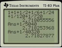
 gives a somewhat more tractable way of approximating
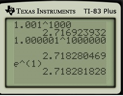
 get very small very quickly, leading to rapid convergence. Indeed, with only terms up to
  , this approximation beats the above approximation with
  . Adding just two extra terms comes close to matching the accuracy of the above limit when
  .
.
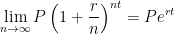
 dollars are invested at interest rate
  for
for  years with continuous compound interest, then the amount of money after
  .
. is equal to
  , so that
 .
.
 .
. .
.![\ln L = \displaystyle \ln \left[ \lim_{n \to \infty} P \left( 1 + \frac{r}{n} \right)^{nt} \right]](https://s0.wp.com/latex.php?latex=%5Cln+L+%3D+%5Cdisplaystyle+%5Cln+%5Cleft%5B+%5Clim_%7Bn+%5Cto+%5Cinfty%7D+P+%5Cleft%28+1+%2B+%5Cfrac%7Br%7D%7Bn%7D+%5Cright%29%5E%7Bnt%7D+%5Cright%5D&bg=ffffff&fg=000000&s=0&c=20201002)
 is continuous, we can
![\ln L = \displaystyle \lim_{n \to \infty} \ln \left[ P \left( 1 + \frac{r}{n} \right)^{nt} \right]](https://s0.wp.com/latex.php?latex=%5Cln+L+%3D+%5Cdisplaystyle+%5Clim_%7Bn+%5Cto+%5Cinfty%7D+%5Cln+%5Cleft%5B+P+%5Cleft%28+1+%2B+%5Cfrac%7Br%7D%7Bn%7D+%5Cright%29%5E%7Bnt%7D+%5Cright%5D&bg=ffffff&fg=000000&s=0&c=20201002)
![\ln L = \displaystyle \lim_{n \to \infty} \left[ \ln P + \ln \left( 1 + \frac{r}{n} \right)^{nt} \right]](https://s0.wp.com/latex.php?latex=%5Cln+L+%3D+%5Cdisplaystyle+%5Clim_%7Bn+%5Cto+%5Cinfty%7D+%5Cleft%5B+%5Cln+P+%2B+%5Cln+%5Cleft%28+1+%2B+%5Cfrac%7Br%7D%7Bn%7D+%5Cright%29%5E%7Bnt%7D+%5Cright%5D&bg=ffffff&fg=000000&s=0&c=20201002)
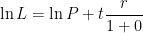
![\ln L = \displaystyle \lim_{n \to \infty} \left[ \ln P + nt \ln \left( 1 + \frac{r}{n} \right)\right]](https://s0.wp.com/latex.php?latex=%5Cln+L+%3D+%5Cdisplaystyle+%5Clim_%7Bn+%5Cto+%5Cinfty%7D+%5Cleft%5B+%5Cln+P+%2B+nt+%5Cln+%5Cleft%28+1+%2B+%5Cfrac%7Br%7D%7Bn%7D+%5Cright%29%5Cright%5D&bg=ffffff&fg=000000&s=0&c=20201002)


 , as so we may apply L’Hopital’s Rule. Taking the derivative of both the numerator and denominator with respect to
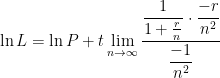


 :
:


 and
and 
 .
.
 with
with  with
with  . Then we obtain

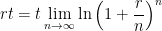

![rt = \displaystyle \lim_{n \to \infty} \ln \left[ \left(1 + \frac{r}{n} \right)^{n} \right]^t](https://s0.wp.com/latex.php?latex=rt+%3D+%5Cdisplaystyle+%5Clim_%7Bn+%5Cto+%5Cinfty%7D+%5Cln+%5Cleft%5B+%5Cleft%281+%2B+%5Cfrac%7Br%7D%7Bn%7D+%5Cright%29%5E%7Bn%7D+%5Cright%5D%5Et&bg=ffffff&fg=000000&s=0&c=20201002)
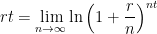
![rt = \displaystyle \ln \left[ \lim_{n \to \infty} \left(1 + \frac{r}{n} \right)^{nt} \right]](https://s0.wp.com/latex.php?latex=rt+%3D+%5Cdisplaystyle+%5Cln+%5Cleft%5B+%5Clim_%7Bn+%5Cto+%5Cinfty%7D+%5Cleft%281+%2B+%5Cfrac%7Br%7D%7Bn%7D+%5Cright%29%5E%7Bnt%7D+%5Cright%5D&bg=ffffff&fg=000000&s=0&c=20201002)

 .
. .
.![\ln L = \displaystyle \ln \left[ \lim_{h \to 0} \left( 1 + h \right)^{1/h} \right]](https://s0.wp.com/latex.php?latex=%5Cln+L+%3D+%5Cdisplaystyle+%5Cln+%5Cleft%5B+%5Clim_%7Bh+%5Cto+0%7D+%5Cleft%28+1+%2B+h+%5Cright%29%5E%7B1%2Fh%7D+%5Cright%5D&bg=ffffff&fg=000000&s=0&c=20201002)


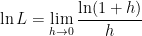
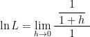

 .
. .
. .
. :
:


![e^1 = \exp \left[ \displaystyle \lim_{h \to 0} \ln (1 + h)^{1/h} \right]](https://s0.wp.com/latex.php?latex=e%5E1+%3D+%5Cexp+%5Cleft%5B+%5Cdisplaystyle+%5Clim_%7Bh+%5Cto+0%7D+%5Cln+%281+%2B+h%29%5E%7B1%2Fh%7D+%5Cright%5D&bg=ffffff&fg=000000&s=0&c=20201002)
 is continuous, we can
![e = \displaystyle \lim_{h \to 0} \exp \left[ \ln (1 + h)^{1/h} \right]](https://s0.wp.com/latex.php?latex=e+%3D+%5Cdisplaystyle+%5Clim_%7Bh+%5Cto+0%7D+%5Cexp+%5Cleft%5B+%5Cln+%281+%2B+h%29%5E%7B1%2Fh%7D+%5Cright%5D&bg=ffffff&fg=000000&s=0&c=20201002)
 .
. .
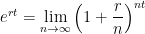
. for
for  becomes
  . Also, as
  , then
  .
. for computing the value of an investment when interest is compounded
  as
as  .
. instead of
  . In this way, we can think like an
  . Then the discrete compound interest formula becomes
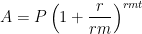

![A = P\displaystyle \left[ \left( 1 + \frac{1}{m} \right)^m \right]^{rt}](https://s0.wp.com/latex.php?latex=A+%3D+P%5Cdisplaystyle+%5Cleft%5B+%5Cleft%28+1+%2B+%5Cfrac%7B1%7D%7Bm%7D+%5Cright%29%5Em+%5Cright%5D%5E%7Brt%7D&bg=ffffff&fg=000000&s=0&c=20201002)
 , except that the name of the variable has changed from
  . But that’s no big deal: as
  and both
 ,
, , so that we can simply replace
  increases as
  .
. ) that earns 100% interest (so that
  ) for one year (so that
  ). This isn’t financially realistic, of course, but let’s run with it. Then the compound interest formula becomes
 , then
  . I’ll usually double-check with my class to make sure that they believe this answer… that $1 compounded once at 100% interest results in $2.
 , then
  .
. , then
  .
. , then
  .
.

 treatment of limit in an honors calculus class or in real analysis. So, mathematically speaking, the above argument should not be considered a proper definition of the number