Inverse Functions: Arcsecant (Part 29)

We now turn to a little-taught and perhaps controversial inverse function: arcsecant. As we’ve seen throughout this series, the domain of this inverse function must be chosen so that the graph of $y = \sec x$ satisfies the horizontal line test. It turns out that the choice of domain has surprising consequences that are almost unforeseeable using only the tools of Precalculus.

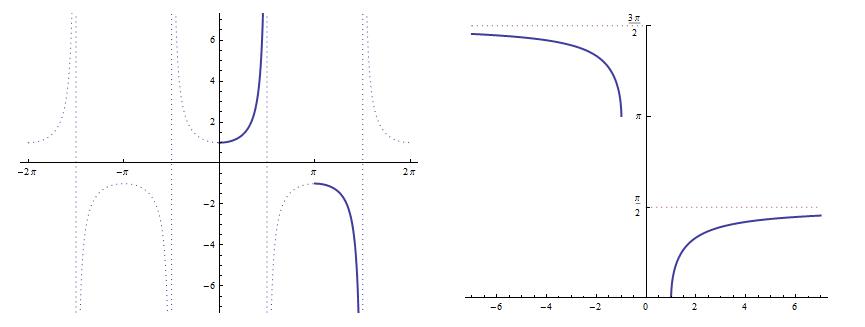
The standard definition of $y = \sec^{-1} x$ uses the interval $[0,\pi]$ — or, more precisely, $[0,\pi/2) \cup (\pi/2, \pi]$ to avoid the vertical asymptote at $x = \pi/2$ — in order to approximately match the range of $\cos^{-1} x$ . However, when I was a student, I distinctly remember that my textbook chose $[0,\pi/2) \cup [\pi,3\pi/2)$ as the range for $\sec^{-1} x$ .

I believe that this definition has fallen out of favor today. However, for the purpose of today’s post, let’s just run with this definition and see what happens. This portion of the graph of $y = \sec x$ is perhaps unorthodox, but it satisfies the horizontal line test so that the inverse function can be defined.

Let’s fast-forward a couple of semesters and use implicit differentiation (see also https://meangreenmath.com/2014/08/08/different-definitions-of-logarithm-part-8/ for how this same logic is used for other inverse functions) to find the derivative of $y = \sec^{-1} x$ :

$x = \sec y$

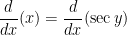
$\displaystyle \frac{d}{dx} (x) = \displaystyle \frac{d}{dx} (\sec y)$

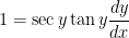
$1 = \sec y \tan y \displaystyle \frac{dy}{dx}$

$\displaystyle \frac{1}{\sec y \tan y} = \displaystyle \frac{dy}{dx}$

At this point, the object is to convert the left-hand side to something involving only $x$ . Clearly, we can replace $\sec y$ with $x$ . As it turns out, the replacement of $\tan y$ is a lot simpler than we saw in yesterday’s post. Once again, we begin with one of the Pythagorean identities:

$1 + \tan^2 y = \sec^2 y$

$\tan^2 y = \sec^2 y - 1$

$\tan^2 y = x^2 - 1$

$\tan y = \sqrt{x^2 - 1} \qquad \hbox{or} \tan y = -\sqrt{x^2 - 1}$

So which is it, the positive answer or the negative answer? In yesterday’s post, the answer depended on whether $x$ was positive or negative. However, with the current definition of $\sec^{-1} x$ , we know for certain that the answer is the positive one! How can we be certain? The angle $y$ must lie in either the interval $[0,\pi/2)$ or else the interval $[\pi,3\pi/2)$ . In either interval, $\tan y$ is positive. So, using this definition of $\sec^{-1} x$ , we can simply say that

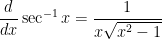
$\displaystyle \frac{d}{dx} \sec^{-1} x = \displaystyle \frac{1}{x \sqrt{x^2-1}}$ ,

and we don’t have to worry about $|x|$ that appeared in yesterday’s post.

Turning to integration, we now have the simple formula

$\displaystyle \int \frac{dx}{x \sqrt{x^2 -1}} = \sec^{-1} x + C$

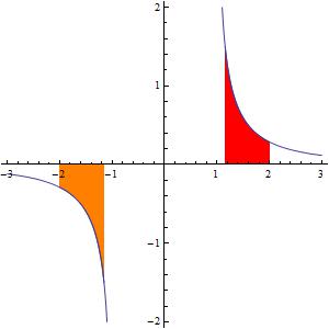
that works whether $x$ is positive or negative. For example, the orange area can now be calculated correctly:

$\displaystyle \int_{-2}^{-2\sqrt{3}/3} \frac{dx}{x \sqrt{x^2 -1}} = \sec^{-1} \left( - \displaystyle \frac{2\sqrt{3}}{3} \right) - \sec^{-1} (-2)$

$= \displaystyle \frac{7\pi}{6} - \frac{4\pi}{3}$

$= \displaystyle -\frac{\pi}{6}$

So, unlike yesterday’s post, this definition of $\sec^{-1} x$ produces a simple integration formula.

So why isn’t this the standard definition for $\sec^{-1} x$ ? I’m afraid the answer is simple: with this definition, the equation

$\sec^{-1} x = \cos^{-1} \left( \displaystyle \frac{1}{x} \right)$

is no longer correct if $x < -1$ . Indeed, I distinctly remember thinking, back when I was a student taking trigonometry, that the definition of $\sec^{-1} x$ seemed really odd, and it seemed to me that it would be better if it matched that of $\cos^{-1} x$ . Of course, at that time in my mathematical development, it would have been almost hopeless to explain that the range $[0,\pi/2) \cup [\pi,3\pi/2)$ had been chosen to simplify certain integrals from calculus.

So I suppose that The Powers That Be have decided that it’s more important for this identity to hold than to have a simple integration formula for $\displaystyle \int \frac{dx}{x \sqrt{x^2 -1}}$

Inverse Functions: Arcsecant (Part 28)

The standard definition of $y = \sec^{-1} x$ uses the interval $[0,\pi]$ , so that

$\sec^{-1} x = \cos^{-1} \left( \displaystyle \frac{1}{x} \right)$

Why would this be controversial? Yesterday, we saw that $\tan x$ is both positive and negative on the interval $[0,\pi]$ , and so great care has to be used to calculate the integral:

$\displaystyle \int \frac{dx}{x \sqrt{x^2 -1}}$

Here’s another example: let’s use trigonometric substitution to calculate

$\displaystyle \int_{-6}^{-3} \frac{ \sqrt{x^2-9} }{x} dx$

The standard trick is to use the substitution $x = 3 \sec \theta$ . With this substitution:

$x^2 - 9 = 9 \sec^2 \theta - 9 = 9 \tan^2 \theta$ , and
$dx = 3 \sec \theta \tan \theta \, d\theta$
$x = -3 \quad \Longrightarrow \quad \sec \theta = -1 \quad \Longrightarrow \quad \theta = \sec^{-1} (-1) = \pi$
$x = -6 \quad \Longrightarrow \quad \sec \theta = -2 \quad \Longrightarrow \quad \theta = \sec^{-1} (-2) = \displaystyle \frac{2\pi}{3}$

Therefore,

$\displaystyle \int_{-6}^{-3} \frac{ \sqrt{x^2-9} }{x} dx = \displaystyle \int_{2\pi/3}^{\pi} \frac{ \sqrt{9 \tan^2 \theta}} { 3 \sec \theta} 3 \sec \theta \tan \theta \, d\theta$

At this point, the common mistake would be to replace $\sqrt{9 \tan^2 \theta}$ with $3 \tan \theta$ . This is a mistake because

$\sqrt{9 \tan^2 \theta} = |3 \tan \theta|$

Furthermore, for this particular problem, $\tan \theta$ is negative on the interval $[2\pi/3,\pi]$ . Therefore, for this problem, we should replace $\sqrt{9 \tan^2 \theta}$ with $-3 \tan \theta$ .

Continuing the calculation,

$\displaystyle \int_{-6}^{-3} \frac{ \sqrt{x^2-9} }{x} dx = \displaystyle \int_{2\pi/3}^{\pi} \frac{ -3 \tan \theta} { 3 \sec \theta} 3 \sec \theta \tan \theta$

$= \displaystyle \int_{2\pi/3}^{\pi} -3\tan^2 \theta \, d\theta$

$= \displaystyle \int_{2\pi/3}^{\pi} -3(\sec^2 \theta-1) \, d\theta$

$= \displaystyle \int_{2\pi/3}^{\pi} (3-3 \sec^2 \theta) \, d\theta$

$= \displaystyle \bigg[ 3 \theta - 3 \tan \theta \bigg]_{2\pi/3}^{\pi}$

$= \displaystyle \left[ 3 \pi - 3 \tan \pi \right] - \left[ 3 \left( \frac{2\pi}{3} \right) - 3 \tan \left( \frac{2\pi}{3} \right) \right]$

$= \displaystyle 3\pi - 0 - 2\pi + 3(-\sqrt{3})$

$= \pi - 3\sqrt{3}$

So if great care wasn’t used to correctly simplify $\sqrt{9 \tan^2 \theta}$ , one would instead obtain the incorrect answer $3\sqrt{3} - \pi$ .

Inverse Functions: Arcsecant (Part 27)

The standard definition of $y = \sec^{-1} x$ uses the interval $[0,\pi]$ , so that

$\sec^{-1} x = \cos^{-1} \left( \displaystyle \frac{1}{x} \right)$

Why would this be controversial? Let’s fast-forward a couple of semesters and use implicit differentiation (see also https://meangreenmath.com/2014/08/08/different-definitions-of-logarithm-part-8/ for how this same logic is used for other inverse functions) to find the derivative of $y = \sec^{-1} x$ :

$x = \sec y$

$\displaystyle \frac{d}{dx} (x) = \displaystyle \frac{d}{dx} (\sec y)$

$1 = \sec y \tan y \displaystyle \frac{dy}{dx}$

$\displaystyle \frac{1}{\sec y \tan y} = \displaystyle \frac{dy}{dx}$

At this point, the object is to convert the left-hand side to something involving only $x$ . Clearly, we can replace $\sec y$ with $x$ . However, doing the same with $\tan y$ is trickier. We begin with one of the Pythagorean identities:

$1 + \tan^2 y = \sec^2 y$

$\tan^2 y = \sec^2 y - 1$

$\tan^2 y = x^2 - 1$

$\tan y = \sqrt{x^2 - 1} \qquad \hbox{or} \tan y = -\sqrt{x^2 - 1}$

So which is it, the positive answer or the negative answer? The answer is, without additional information, we don’t know!

If $0 \le y < \pi/2$ (so that $x = \sec y \ge 1$ ), then $\tan y$ is positive, and so $\tan y = \sqrt{\sec^2 y - 1}$ .
If $\pi/2 < y \le \pi$ (so that $x = \sec y \le 1$ ), then $\tan y$ is negative, and so $\tan y = -\sqrt{\sec^2 y - 1}$ .

We therefore have two formulas for the derivative of $y = \sec^{-1} x$ :

$\displaystyle \frac{d}{dx} sec^{-1} x = \displaystyle \frac{1}{x \sqrt{x^2-1}} \qquad \hbox{if} \qquad x > 1$

$\displaystyle \frac{d}{dx} sec^{-1} x = \displaystyle -\frac{1}{x \sqrt{x^2-1}} \qquad \hbox{if} \qquad x < 1$

These may then be combined into the single formula

$\displaystyle \frac{d}{dx} sec^{-1} x = \displaystyle \frac{1}{|x| \sqrt{x^2-1}}$

It gets better. Let’s now find the integral

$\displaystyle \int \frac{dx}{x \sqrt{x^2 -1}}$

Several calculus textbooks that I’ve seen will lazily give the answer

$\displaystyle \int \frac{dx}{x \sqrt{x^2 -1}} = \sec^{-1} x + C$

This answer works as long as $x > 1$ , so that $|x|$ reduces to simply $x$ . For example, the red signed area in the above picture on the interval $[2\sqrt{3}/3,2]$ may be correctly computed as

$\displaystyle \int_{2\sqrt{3}/3}^2 \frac{dx}{x \sqrt{x^2 -1}} = \sec^{-1} 2 - \sec^{-1} \displaystyle \frac{2\sqrt{3}}{3}$

$= \cos^{-1} \left( \displaystyle \frac{1}{2} \right) - \cos^{-1} \left( \displaystyle \frac{\sqrt{3}}{2} \right)$

$= \displaystyle \frac{\pi}{3} - \frac{\pi}{6}$

$= \displaystyle \frac{\pi}{6}$

However, the orange signed area on the interval $[-2,-2\sqrt{3}/3]$ is incorrectly computed using this formula!

$\displaystyle \int_{-2}^{-2\sqrt{3}/3} \frac{dx}{x \sqrt{x^2 -1}} = \sec^{-1} \left( - \displaystyle \frac{2\sqrt{3}}{3} \right) - \sec^{-1} (-2)$

$= \cos^{-1} \left( -\displaystyle \frac{\sqrt{3}}{2} \right) -\cos^{-1} \left( \displaystyle \frac{1}{2} \right)$

$= \displaystyle \frac{5\pi}{6} - \frac{2\pi}{3}$

$= \displaystyle \frac{\pi}{6}$

This is patently false, as the picture clearly indicates that the above integral has to be negative. For this reason, careful calculus textbooks will often ask students to solve a problem like

$\displaystyle \int \frac{dx}{x \sqrt{x^2 -1}}, \qquad x > 1$

and the caveat $x > 1$ is needed to ensure that the correct antiderivative is used. Indeed, a calculus textbook that doesn’t include such caveats are worthy of any scorn that an instructor cares to heap upon it.

Inverse Functions: Arcsecant (Part 26)

The standard definition of $y = \sec^{-1} x$ uses the interval $[0,\pi]$ — or, more precisely, $[0,\pi/2) \cup (\pi/2, \pi]$ to avoid the vertical asymptote at $x = \pi/2$ . This portion of the graph of $y = \sec x$ satisfies the horizontal line test and, conveniently, matches almost perfectly the domain of $y = \cos^{-1} x$ . This is perhaps not surprising since, when both are defined, $\cos x$ and $\sec x$ are reciprocals.

Since this range of $\sec^{-1} x$ matches that of $\cos^{-1} x$ , we have the convenient identity

$\sec^{-1} x = \cos^{-1} \left( \displaystyle \frac{1}{x} \right)$

To see why this works, let’s examine the right triangle below. Notice that

$\cos \theta = \displaystyle \frac{x}{1} \qquad \Longrightarrow \qquad \theta = \cos^{-1} x$ .

Also,

$\sec\theta = \displaystyle \frac{1}{x} \qquad \Longrightarrow \qquad \theta = \cos^{-1} \left( \displaystyle \frac{1}{x} \right)$ .

This argument provides the justification for $0 < \theta < \pi/2$ — that is, for $x > 1$ — but it still works for $x = 1$ and $x \le -1$ .

So this seems like the most natural definition in the world for $\sec^{-1} x$ . Unfortunately, there are consequences for this choice in calculus, as we’ll see in tomorrow’s post.

Exponential growth and decay (Part 16): Logistic growth model

In this series of posts, I provide a deeper look at common applications of exponential functions that arise in an Algebra II or Precalculus class. In the previous posts in this series, I considered financial applications, radioactive decay, and Newton’s Law of Cooling.

Today, I discuss the logistic growth model, which describes how an infection (like a disease, a rumor, or advertise) spreads in a population. In yesterday’s post, I described an in-class demonstration that engages students while also making the following formula believable:

$A(t) = \displaystyle \frac{Ly_0}{y_0+ (L-y_0)e^{-rt}}$ .

I’d like to discuss some observations about this somewhat complicated function that will make producing its graph easier. The first two observations are within reach of Precalculus students.

1. Let’s figure out the $y-$ intercept:

$A(0) = \displaystyle \frac{Ly_0}{y_0+ (L-y_0)e^{-r \cdot 0}} = \displaystyle \frac{Ly_0}{y_0+ L-y_0} = y_0$ .

In other words, the number $y_0$ represents the initial number of people who have the infection.

2. Let’s figure out the limiting value as $t$ gets large:

$\displaystyle \lim_{t \to \infty} A(t) = \displaystyle \frac{Ly_0}{y_0+ (L-y_0) \cdot 0} = \displaystyle \frac{Ly_0}{y_0} = L$ .

As expected, all $L$ people will get the infection eventually. (Of course, Precalculus students won’t be familiar with the $\displaystyle \lim$ notation, but they should understand that $e^{-rt}$ decays to zero as $t$ gets large.

3. Let’s now figure out the point of inflection. Ordinarily, points of inflection are found by setting the second derivative equal to zero. Though this can be done for the function $A(t)$ above, it would be a somewhat daunting exercise!

The good news is that the points of inflection can be found quite simply using the governing differential equation, which is

$A' = r A [ L - A] = r L A - r A^2$

Let’s take the derivative of both sides, remembering that $r$ and $L$ are constants:

$A'' = r L A' - 2 r A A'$

$A'' = A' (r L - 2 r A)$

So the second derivative is equal to zero when either $A' = 0$ or else $r L - 2 r A = 0$ . The first case corresponds to the trivial cases $A(t) \equiv 0$ and $A(t) \equiv L$ ; these constants are called the equilibrium solutions. The second case is the more interesting one:

$r L - 2 r A = 0$

$r L = 2 r A$

$\displaystyle \frac{L}{2} = A$

This suggests that, as the infection spreads throughout a population, the curve changes concavity at the time that half of the population becomes infected. In other words, the infection spreads fastest throughout the population at the time when half of the population has been infected.

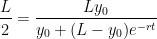
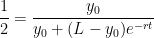
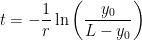
The time at which the point of inflection occurs can be found by setting $A(t) = \displaystyle \frac{L}{2}$ and solving for $t$ :

$\displaystyle \frac{L}{2} = \displaystyle \frac{Ly_0}{y_0+ (L-y_0)e^{-rt}}$ .

$\displaystyle \frac{1}{2} = \displaystyle \frac{y_0}{y_0+ (L-y_0)e^{-rt}}$ .

$y_0 + (L-y_0) e^{-rt} = 2y_0$

$(L-y_0) e^{-rt} = y_0$

$e^{-rt} = \displaystyle \frac{y_0}{L-y_0}$

$-rt = \displaystyle \ln \left( \frac{y_0}{L-y_0} \right)$

$t = \displaystyle - \frac{1}{r} \ln \left( \frac{y_0}{L-y_0} \right)$

This technique for finding the points of inflection directly from the differential equation is possible whenever the differential equation is autonomous, which loosely means that the independent variable does not appear on the right-hand side.

Different definitions of e (Part 12): Numerical computation

In this series of posts, we have seen that the number $e$ can be thought about in three different ways.

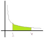
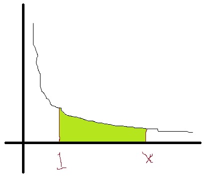
1. $e$ defines a region of area 1 under the hyperbola $y = 1/x$ .2. We have the limits

$e = \displaystyle \lim_{h \to 0} (1+h)^{1/h} = \displaystyle \lim_{n \to \infty} \left(1 + \frac{1}{n} \right)^n$ .

These limits form the logical basis for the continuous compound interest formula.

3. We have also shown that $\frac{d}{dx} \left(e^x \right) = e^x$ . From this derivative, the Taylor series expansion for $e^x$ about $x = 0$ can be computed:

$e^x = \displaystyle \sum_{n=0}^\infty \frac{x^n}{n!}$

Therefore, we can let $x = 1$ to find $e$ :

$e = \displaystyle \sum_{n=0}^\infty \frac{1}{n!} = \displaystyle 1 + 1 + \frac{1}{2} + \frac{1}{6} + \frac{1}{24} + \dots$

In yesterday’s post, I showed that using the original definition (in terms of an area under a hyperbola) does not lend itself well to numerically approximating $e$ . Let’s now look at the other two methods.

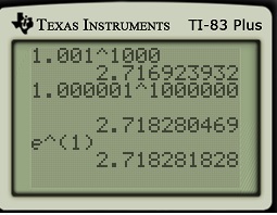
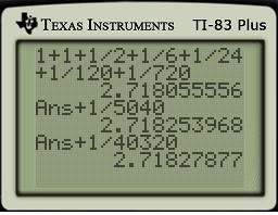
2. The limit $e = \displaystyle \lim_{n \to \infty} \left(1 + \frac{1}{n} \right)^n$ gives a somewhat more tractable way of approximating $e$ , at least with a modern calculator. However, you can probably imagine the fun of trying to use this formula without a calculator.

3. The best way to compute $e$ (or, in general, $e^x$ ) is with Taylor series. The fractions $\frac{1}{n!}$ get very small very quickly, leading to rapid convergence. Indeed, with only terms up to $1/6!$ , this approximation beats the above approximation with $n = 1000$ . Adding just two extra terms comes close to matching the accuracy of the above limit when $n = 1,000,000$ .

More about approximating $e^x$ via Taylor series can be found in my previous post.

Different definitions of e (Part 10): Connecting the two definitions

In this series of posts, I consider how two different definitions of the number $e$ are related to each other. The number $e$ is usually introduced at two different places in the mathematics curriculum:

Algebra II/Precalculus: If $P$ dollars are invested at interest rate $r$ for $t$ years with continuous compound interest, then the amount of money after $t$ years is $A = Pe^{rt}$ .
Calculus: The number $e$ is defined to be the number so that the area under the curve $y = 1/x$ from $x = 1$ to $x = e$ is equal to $1$ , so that

$\displaystyle \int_1^e \frac{dx}{x} = 1$ .

These two definitions appear to be very, very different. One deals with making money. The other deals with the area under a hyperbola. Amazingly, these two definitions are related to each other. In this series of posts, I’ll discuss the connection between the two.

In yesterday’s post, I proved the following theorem, thus completing a long train of argument that began with the second definition of $e$ and ending with a critical step in the derivation of the continuous compound interest formula. Today, I present an alternate proof of the theorem using L’Hopital’s rule.

Theorem. $\displaystyle \lim_{n \to \infty} P \left( 1 + \frac{r}{n} \right)^{nt} = P e^{rt}$ .

Proof #2. Let’s write the left-hand side as

$L = \displaystyle \lim_{n \to \infty} P \left( 1 + \frac{r}{n} \right)^{nt}$ .

Let’s take the natural logarithm of both sides:

$\ln L = \displaystyle \ln \left[ \lim_{n \to \infty} P \left( 1 + \frac{r}{n} \right)^{nt} \right]$

Since $g(x) = \ln x$ is continuous, we can interchange the function and the limit on the right-hand side:

$\ln L = \displaystyle \lim_{n \to \infty} \ln \left[ P \left( 1 + \frac{r}{n} \right)^{nt} \right]$

$\ln L = \displaystyle \lim_{n \to \infty} \left[ \ln P + \ln \left( 1 + \frac{r}{n} \right)^{nt} \right]$

$\ln L = \displaystyle \lim_{n \to \infty} \left[ \ln P + nt \ln \left( 1 + \frac{r}{n} \right)\right]$

$\ln L = \ln P + \displaystyle \lim_{n \to \infty} \frac{t \displaystyle \ln \left(1 + \frac{r}{n} \right)}{1/n}$

$\ln L = \ln P + \displaystyle t \lim_{n \to \infty} \frac{\displaystyle \ln \left(1 + \frac{r}{n} \right)}{1/n}$

The limit on the right-hand side follows the indeterminate form $0/0$ , as so we may apply L’Hopital’s Rule. Taking the derivative of both the numerator and denominator with respect to $n$ , we find

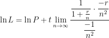
$\ln L = \ln P + \displaystyle t \lim_{n \to \infty} \frac{\displaystyle \frac{1}{1 + \frac{r}{n}} \cdot \frac{-r}{n^2}}{\displaystyle \frac{-1}{n^2}}$

$\ln L = \ln P + \displaystyle t \lim_{n \to \infty}\frac{r}{1 + \frac{r}{n}}$

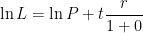
$\ln L = \ln P + \displaystyle t \frac{r}{1 + 0}$

$\ln L = rt + \ln P$

We now solve for the original limit $L$ :

$L = e^{rt + \ln P}$

$L = e^{rt} e^{\ln P}$

$L = Pe^{rt}$

Different definitions of e (Part 9): Connecting the two definitions

Algebra II/Precalculus: If $P$ dollars are invested at interest rate $r$ for $t$ years with continuous compound interest, then the amount of money after $t$ years is $A = Pe^{rt}$ .
Calculus: The number $e$ is defined to be the number so that the area under the curve $y = 1/x$ from $x = 1$ to $x = e$ is equal to $1$ , so that

$\displaystyle \int_1^e \frac{dx}{x} = 1$ .

We begin with the second definition, which is usually considered the true definition of $e$ . From this definition, I have shown in a previous post that we can derive the differentiation formulas

$\displaystyle \frac{d}{dx} (\ln x) = \frac{1}{x} \qquad$ and $\qquad \displaystyle \frac{d}{dx} \left( e^x \right) = e^x$

beginning with this definition of the number $e$ .

Theorem. $\displaystyle \lim_{n \to \infty} P \left( 1 + \frac{r}{n} \right)^{nt} = Pe^{rt}$ .

Proof #1.In an earlier post in this series, I showed that

$\displaystyle \frac{1}{x} = \displaystyle \lim_{h \to 0} \ln \left(1 + \frac{h}{x} \right)^{1/h}$

Let’s now replace $h$ with $1/n$ . Also, replace $x$ with $1/r$ . Then we obtain

$r = \displaystyle \lim_{n \to \infty} \ln \left(1 + \frac{1/n}{1/r} \right)^{n}$

$r = \displaystyle \lim_{n \to \infty} \ln \left(1 + \frac{r}{n} \right)^{n}$

Multiply both sides by $t$ :

$rt = \displaystyle t \lim_{n \to \infty} \ln \left(1 + \frac{r}{n} \right)^{n}$

$rt = \displaystyle \lim_{n \to \infty} t \ln \left(1 + \frac{r}{n} \right)^{n}$

$rt = \displaystyle \lim_{n \to \infty} \ln \left[ \left(1 + \frac{r}{n} \right)^{n} \right]^t$

$rt = \displaystyle \lim_{n \to \infty} \ln \left(1 + \frac{r}{n} \right)^{nt}$

Since $g(x) = \ln x$ is continuous, we can interchange the function and the limit on the right-hand side:

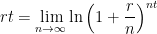
$rt = \displaystyle \ln \left[ \lim_{n \to \infty} \left(1 + \frac{r}{n} \right)^{nt} \right]$

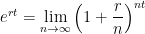
$e^{rt} = \displaystyle \lim_{n \to \infty} \left(1 + \frac{r}{n} \right)^{nt}$

Finally, we multiply both sides by $P$ :

$P e^{rt} = \displaystyle \lim_{n \to \infty} P \left(1 + \frac{r}{n} \right)^{nt}$

(A second proof of this theorem, using L’Hopital’s Rule, will be presented in tomorrow’s post.)

This firmly established, at last, the connection between the continuous compound interest formula and the area under the hyperbola. I’ve noted that my students feel a certain sense of accomplishment after reaching this point of the exposition.

Different definitions of e (Part 8): Connecting the two definitions

Algebra II/Precalculus: If $P$ dollars are invested at interest rate $r$ for $t$ years with continuous compound interest, then the amount of money after $t$ years is $A = Pe^{rt}$ .
Calculus: The number $e$ is defined to be the number so that the area under the curve $y = 1/x$ from $x = 1$ to $x = e$ is equal to $1$ , so that

$\displaystyle \int_1^e \frac{dx}{x} = 1$ .

Theorem. $\displaystyle \lim_{h \to 0} \left( 1 + h \right)^{1/h} = e$ .

Proof #2. Let’s write the left-hand side as

$L = \displaystyle \lim_{h \to 0} \left( 1 + h \right)^{1/h}$ .

Let’s take the natural logarithm of both sides:

$\ln L = \displaystyle \ln \left[ \lim_{h \to 0} \left( 1 + h \right)^{1/h} \right]$

Since $g(x) = \ln x$ is continuous, we can interchange the function and the limit on the right-hand side:

$\ln L = \displaystyle \lim_{h \to 0} \ln (1+h)^{1/h}$

$\ln L = \displaystyle \lim_{h \to 0} \frac{1}{h} \ln(1+h)$

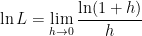
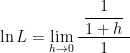
$\ln L = \displaystyle \lim_{h \to 0} \frac{\ln(1+h)}{h}$

The right-hand side follows the indeterminate form $0/0$ , as so we may apply L’Hopital’s Rule. Taking the derivative of both the numerator and denominator, we find

$\ln L = \displaystyle \lim_{h \to 0} \frac{ \displaystyle ~ \frac{1}{1+h} ~}{1}$

$\ln L = \displaystyle \lim_{h \to 0} \frac{1}{1+h}$

$\ln L = \displaystyle \frac{1}{1+0} = 1$ .

Therefore, the original limit is $L = e^1 = e$ .

Different definitions of e (Part 7): Connecting the two definitions

Algebra II/Precalculus: If $P$ dollars are invested at interest rate $r$ for $t$ years with continuous compound interest, then the amount of money after $t$ years is $A = Pe^{rt}$ .
Calculus: The number $e$ is defined to be the number so that the area under the curve $y = 1/x$ from $x = 1$ to $x = e$ is equal to $1$ , so that

$\displaystyle \int_1^e \frac{dx}{x} = 1$ .

We begin with the second definition, which is usually considered the true definition of $e$ . From this definition, I have shown in a previous post that we can derive the differentiation formulas

$\displaystyle \frac{d}{dx} (\ln x) = \frac{1}{x} \qquad$ and $\qquad \displaystyle \frac{d}{dx} \left( e^x \right) = e^x$

beginning with this definition of the number $e$ .

Theorem. $\displaystyle \lim_{h \to 0} \left( 1 + h \right)^{1/h} = e$ .

Proof #1. Recall the definition of a derivative

$f'(x) = \displaystyle \lim_{h \to 0} \frac{f(x+h) - f(x)}{h}$ .

Let’s apply this to the function $f(x) = \ln x$ :

$\displaystyle \frac{d}{dx} (\ln x) = \displaystyle \lim_{h \to 0} \frac{\ln(x+h) - \ln x}{h}$

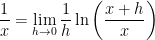
$\displaystyle \frac{1}{x} = \displaystyle \lim_{h \to 0} \frac{1}{h} \ln \left( \frac{x+h}{x} \right)$

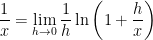
$\displaystyle \frac{1}{x} = \displaystyle \lim_{h \to 0} \frac{1}{h} \ln \left( 1 + \frac{h}{x} \right)$

$\displaystyle \frac{1}{x} = \displaystyle \lim_{h \to 0} \ln \left(1 + \frac{h}{x} \right)^{1/h}$

(I’ll note parenthetically that I’ll need the above line for a future post in this series.) At this point, let’s substitute $x = 1$ :

$1 = \displaystyle \lim_{h \to 0} \ln (1 + h)^{1/h}$

Let’s now apply the exponential function to both sides:

$e^1 = \exp \left[ \displaystyle \lim_{h \to 0} \ln (1 + h)^{1/h} \right]$

Since $g(x) = e^x$ is continuous, we can interchange the function and the limit on the right-hand side:

$e = \displaystyle \lim_{h \to 0} \exp \left[ \ln (1 + h)^{1/h} \right]$

Finally, since $g(x) = e^x$ and $f(x) = \ln x$ are inverse functions, we can conclude

$e = \displaystyle \lim_{h \to 0} (1 + h)^{1/h}$ .

(A second proof of this theorem, using L’Hopital’s Rule, will be presented in tomorrow’s post.)

The next theorem establishes, at last, the connection between the continuous compound interest formula and the area under the hyperbola. I’ve noted that my students feel a certain sense of accomplishment after reaching this point of the exposition.

Theorem. $\displaystyle \lim_{n \to \infty} \left(1 + \frac{1}{n} \right)^{n} = e$ .

Proof. Though a little bit of real analysis is necessary to make this rigorous, we can informally see why this has to be true by letting $n = 1/h$ for $h$ positive. Then the expression $(1+h)^{1/h}$ becomes $\left( 1 + \frac{1}{n} \right)^n$ . Also, as $h \to 0$ , then $n \to \infty$ .