Source: https://twitter.com/msurd/status/669651056637272064/photo/1
I’m doing something that I should have done a long time ago: collecting a series of posts into one single post. The following links comprised my series on different ways of computing the limit
Part 1: Algebra
Part 2: L’Hopital’s Rule
Part 3: Trigonometric substitution
Part 4: Geometry
Part 5: Geometry again
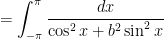
This series was inspired by a question that my wife asked me: calculate
 and performed a substitution. However, as I’ve discussed in this series, there are four different ways that this integral can be evaluated.
 Since
Since 


![= 2\pi i \left[\displaystyle \frac{r_1}{r_1^2-1} + \displaystyle \frac{r_2}{r_2^2-1} \right]](https://s0.wp.com/latex.php?latex=%3D+2%5Cpi+i+%5Cleft%5B%5Cdisplaystyle+%5Cfrac%7Br_1%7D%7Br_1%5E2-1%7D+%2B+%5Cdisplaystyle+%5Cfrac%7Br_2%7D%7Br_2%5E2-1%7D+%5Cright%5D&bg=ffffff&fg=000000&s=0&c=20201002)
where I’ve made the assumption that 


Also,
and
are the two poles of the final integrand that lie within this contour.
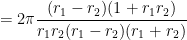
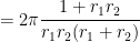
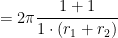
It now remains to simplify the final algebraic expression. To begin, I note

Similarly,
Therefore,
![Q = 2\pi i \left[\displaystyle \frac{r_1}{r_1^2-1} + \displaystyle \frac{r_2}{r_2^2-1} \right] = 2\pi i \left[ \displaystyle \frac{1}{2|b|i} + \frac{1}{2|b| i} \right] = 2\pi i \displaystyle \frac{2}{2|b|i} = \displaystyle \frac{2\pi}{|b|}](https://s0.wp.com/latex.php?latex=Q+%3D+2%5Cpi+i+%5Cleft%5B%5Cdisplaystyle+%5Cfrac%7Br_1%7D%7Br_1%5E2-1%7D+%2B+%5Cdisplaystyle+%5Cfrac%7Br_2%7D%7Br_2%5E2-1%7D+%5Cright%5D+%3D+2%5Cpi+i+%5Cleft%5B+%5Cdisplaystyle+%5Cfrac%7B1%7D%7B2%7Cb%7Ci%7D+%2B+%5Cfrac%7B1%7D%7B2%7Cb%7C+i%7D+%5Cright%5D+%3D+2%5Cpi+i+%5Cdisplaystyle+%5Cfrac%7B2%7D%7B2%7Cb%7Ci%7D+%3D+%5Cdisplaystyle+%5Cfrac%7B2%5Cpi%7D%7B%7Cb%7C%7D&bg=ffffff&fg=000000&s=0&c=20201002)
And so, at long last, I’ve completed a fifth different evaluation of
This series was inspired by a question that my wife asked me: calculate
and performed a substitution. However, as I’ve discussed in this series, there are four different ways that this integral can be evaluated.Since

where
Amazingly, contour integrals can be simply computed by evaluating the residues at every pole located inside of the contour. (See Wikipedia and Mathworld for more details.) I have already handled the case of 

Earlier in this series, I showed that
if


Of these, only two lie (


As shown earlier in this series, the residue at each pole is given by
I’ll now simplify this considerably by using the fact that 

Therefore, to evaluate the contour integral, I simply the sum of the residues within the contour and multiply the sum by 
![Q = \displaystyle \lim_{R \to \infty} \oint_{C_R} \frac{ 2(1+z^2) dz}{z^4 + (4 b^2 - 2) z^2 + 1} = 2\pi i \left[\displaystyle \frac{r_1}{r_1^2-1} + \displaystyle \frac{r_2}{r_2^2-1} \right]](https://s0.wp.com/latex.php?latex=Q+%3D+%5Cdisplaystyle+%5Clim_%7BR+%5Cto+%5Cinfty%7D+%5Coint_%7BC_R%7D+%5Cfrac%7B+2%281%2Bz%5E2%29+dz%7D%7Bz%5E4+%2B+%284+b%5E2+-+2%29+z%5E2+%2B+1%7D+%3D+2%5Cpi+i+%5Cleft%5B%5Cdisplaystyle+%5Cfrac%7Br_1%7D%7Br_1%5E2-1%7D+%2B+%5Cdisplaystyle+%5Cfrac%7Br_2%7D%7Br_2%5E2-1%7D+%5Cright%5D&bg=ffffff&fg=000000&s=0&c=20201002)
So, to complete the evaluation of
This series was inspired by a question that my wife asked me: calculate
and performed a substitution. However, as I’ve discussed in this series, there are four different ways that this integral can be evaluated. nvenient value of
where I’ve assumed
and the positive constants


Now we have the small matter of simplifying our expression for

Fortunately, humans can still do some things that computers can’t. As observed yesterday, The numbers 


These relationships will be very handy for simplifying our expression for
To complete the calculation, I observe that

so that

Therefore,

In tomorrow’s post, I’ll present another way to simplify this nasty algebraic expression.
This series was inspired by a question that my wife asked me: calculate
and performed a substitution. However, as I’ve discussed in this series, there are four different ways that this integral can be evaluated.Since
where
Amazingly, contour integrals can be simply computed by evaluating the residues at every pole located inside of the contour. (See Wikipedia and Mathworld for more details.) I handled the case of
To find the poles of the integrand, I use the quadratic formula to set the denominator equal to zero:
As shown earlier in this series, the right-hand side is negative if
so that the four poles of the integrand are 


Before starting that task, I notice that

or

or

Matching coefficients, I see that

These will become very handy later in the calculation.
The integrand has the form 

In this case, 


and
Finally, to evaluate the contour integral, I simply the sum of the residues within the contour and then multiply the sum by
So, to complete the evaluation of
Amazingly, the integral below has a simple solution:
Even more amazingly, the integral
So here’s what I have been able to develop to prove that
Earlier in this series, I showed that
Yesterday, I showed used the substitution 

Notice that I’ve written this integral as a function of the parameter 


To do this, I differentiate under the integral sign with respect to 
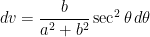
I now apply the trigonometric substitution 
and
The endpoints of integration change from 


I’m not completely thrilled with this demonstration that
and demonstrate that
In a recent class with my future secondary math teachers, we had a fascinating discussion concerning how a teacher should respond to the following question from a student:
Is it ever possible to prove a statement or theorem by proving a special case of the statement or theorem?
Usually, the answer is no. In this series of posts, we’ve seen that a conjecture could be true for the first 40 cases or even the first 
However, there are plenty of examples in mathematics where it is possible to prove a theorem by first proving a special case of the theorem. For the remainder of this series, I’d like to list, in no particular order, some common theorems used in secondary mathematics which are typically proved by first proving a special case.
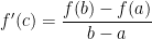
6. Theorem (Mean Value Theorem). If 
![[a,b]](https://s0.wp.com/latex.php?latex=%5Ba%2Cb%5D&bg=ffffff&fg=000000&s=0&c=20201002)


In other words, there is a point 
This is a consequence of the following lemma.
Lemma (Rolle’s Theorem). If 


Notice that Rolle’s Theorem is really a special case of the Mean Value Theorem: if

thus matching the conclusion of Rolle’s Theorem.
I won’t type out the proofs of Rolle’s Theorem and the Mean Value Theorem here, since Wikipedia has already done that very well. Suffice it to say that Rolle’s Theorem logically comes first, and then the Mean Value Theorem can be proven using Rolle’s Theorem. The main idea is to assume that the function
It’s straightforward to show that 

In a recent class with my future secondary math teachers, we had a fascinating discussion concerning how a teacher should respond to the following question from a student:
Is it ever possible to prove a statement or theorem by proving a special case of the statement or theorem?
Usually, the answer is no. In this series of posts, we’ve seen that a conjecture could be true for the first 40 cases or even the first
However, there are plenty of examples in mathematics where it is possible to prove a theorem by first proving a special case of the theorem. For the remainder of this series, I’d like to list, in no particular order, some common theorems used in secondary mathematics which are typically proved by first proving a special case.
5. Theorem. For any rational number 

This theorem is typically proven using the Chain Rule (in the guise of implicit differentiation) and the following lemma:
Lemma. For any integer 

Clearly, the lemma is a special case of the main theorem. However, the lemma can be proven without using the main theorem:
Proof of Lemma (Case 1). If
Case 1 can also be proven using the Product Rule and mathematical induction.
Proof of Lemma (Case 2). If 

Proof of Lemma (Case 3). If 

QED
Now that the lemma has been proven, the main theorem can be proven using the lemma.
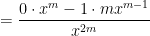
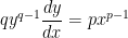
Proof of Theorem. Suppose that 


Let’s now differentiate with respect to
QED
I’m using the Twelve Days of Christmas (and perhaps a few extra days besides) to do something that I should have done a long time ago: collect past series of posts into a single, easy-to-reference post. The following posts formed my series on what I teach my students on the first day of calculus in order to start the transition from Precalculus and to get them engaged for what we’ll be doing throughout the semester.
Part 1: The two themes of calculus: Approximating curved things by straight things and passing to limits.
Part 2: Using the distance-rate-time formula to estimate how fast an accelerating object lands when dropped from a tall building.
Part 3: Passing to limits to precisely calculate the above velocity.
Part 4: Using rectangles to estimate the area under a parabola.
Part 5: Passing to limits to precisely calculate the area under a parabola.
Part 6: Final comments: these two questions apparently have nothing to do with each other, but are in fact highly interrelated. The connection between these two topics, the Fundamental Theorem of Calculus, is one of greatest discoveries in the history of mankind, which my students are now privileged to understand at the ripe old age of 18 or 19 years old.





![\displaystyle \frac{r_1}{r_1^2-1} = \displaystyle \frac{\sqrt{1-b^2} + |b|i}{[\sqrt{1-b^2} + |b|i]^2 - 1}](https://s0.wp.com/latex.php?latex=%5Cdisplaystyle+%5Cfrac%7Br_1%7D%7Br_1%5E2-1%7D+%3D+%5Cdisplaystyle+%5Cfrac%7B%5Csqrt%7B1-b%5E2%7D+%2B+%7Cb%7Ci%7D%7B%5B%5Csqrt%7B1-b%5E2%7D+%2B+%7Cb%7Ci%5D%5E2+-+1%7D&bg=ffffff&fg=000000&s=0&c=20201002)


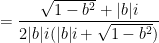
![\displaystyle \frac{r_2}{r_2^2-1} = \displaystyle \frac{-\sqrt{1-b^2} + |b|i}{[-\sqrt{1-b^2} + |b|i]^2 - 1}](https://s0.wp.com/latex.php?latex=%5Cdisplaystyle+%5Cfrac%7Br_2%7D%7Br_2%5E2-1%7D+%3D+%5Cdisplaystyle+%5Cfrac%7B-%5Csqrt%7B1-b%5E2%7D+%2B+%7Cb%7Ci%7D%7B%5B-%5Csqrt%7B1-b%5E2%7D+%2B+%7Cb%7Ci%5D%5E2+-+1%7D&bg=ffffff&fg=000000&s=0&c=20201002)





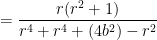


![= 2\pi \displaystyle \left[ \frac{1-r_1^2}{-2r_1^3 + (4b^2-2) r_1} +\frac{1-r_2^2}{-2r_2^3 + (4b^2-2) r_2} \right]](https://s0.wp.com/latex.php?latex=%3D+2%5Cpi+%5Cdisplaystyle+%5Cleft%5B+%5Cfrac%7B1-r_1%5E2%7D%7B-2r_1%5E3+%2B+%284b%5E2-2%29+r_1%7D+%2B%5Cfrac%7B1-r_2%5E2%7D%7B-2r_2%5E3+%2B+%284b%5E2-2%29+r_2%7D+%5Cright%5D&bg=ffffff&fg=000000&s=0&c=20201002)
![Q = 2\pi \displaystyle \left[ \frac{1-r_1^2}{-2r_1^3 + (4b^2-2) r_1} +\frac{1-r_2^2}{-2r_2^3 + (4b^2-2) r_2} \right]](https://s0.wp.com/latex.php?latex=Q+%3D+2%5Cpi+%5Cdisplaystyle+%5Cleft%5B+%5Cfrac%7B1-r_1%5E2%7D%7B-2r_1%5E3+%2B+%284b%5E2-2%29+r_1%7D+%2B%5Cfrac%7B1-r_2%5E2%7D%7B-2r_2%5E3+%2B+%284b%5E2-2%29+r_2%7D+%5Cright%5D&bg=ffffff&fg=000000&s=0&c=20201002)
![= 2\pi \left[ \displaystyle \frac{1-r_1^2}{r_1 (-2r_1^2 + 4b^2-2)} + \frac{1-r_2^2}{r_2(-2r_2^2 + 4b^2-2)} \right]](https://s0.wp.com/latex.php?latex=%3D+2%5Cpi+%5Cleft%5B+%5Cdisplaystyle+%5Cfrac%7B1-r_1%5E2%7D%7Br_1+%28-2r_1%5E2+%2B+4b%5E2-2%29%7D+%2B+%5Cfrac%7B1-r_2%5E2%7D%7Br_2%28-2r_2%5E2+%2B+4b%5E2-2%29%7D+%5Cright%5D&bg=ffffff&fg=000000&s=0&c=20201002)
![= 2\pi \left[ \displaystyle \frac{1-r_1^2}{r_1 (-2r_1^2 +r_1^2 + r_2^2)} + \frac{1-r_2^2}{r_2(-2r_2^2 + r_1^2 + r_2^2)} \right]](https://s0.wp.com/latex.php?latex=%3D+2%5Cpi+%5Cleft%5B+%5Cdisplaystyle+%5Cfrac%7B1-r_1%5E2%7D%7Br_1+%28-2r_1%5E2+%2Br_1%5E2+%2B+r_2%5E2%29%7D+%2B+%5Cfrac%7B1-r_2%5E2%7D%7Br_2%28-2r_2%5E2+%2B+r_1%5E2+%2B+r_2%5E2%29%7D+%5Cright%5D&bg=ffffff&fg=000000&s=0&c=20201002)
![= 2\pi \left[ \displaystyle \frac{1-r_1^2}{r_1 (-r_1^2 +r_2^2)} + \frac{1-r_2^2}{r_2(r_1^2 -r_2^2)} \right]](https://s0.wp.com/latex.php?latex=%3D+2%5Cpi+%5Cleft%5B+%5Cdisplaystyle+%5Cfrac%7B1-r_1%5E2%7D%7Br_1+%28-r_1%5E2+%2Br_2%5E2%29%7D+%2B+%5Cfrac%7B1-r_2%5E2%7D%7Br_2%28r_1%5E2+-r_2%5E2%29%7D+%5Cright%5D&bg=ffffff&fg=000000&s=0&c=20201002)
![= 2\pi \left[ \displaystyle \frac{r_1^2-1}{r_1 (r_1^2 -r_2^2)} + \frac{1-r_2^2}{r_2(r_1^2 -r_2^2)} \right]](https://s0.wp.com/latex.php?latex=%3D+2%5Cpi+%5Cleft%5B+%5Cdisplaystyle+%5Cfrac%7Br_1%5E2-1%7D%7Br_1+%28r_1%5E2+-r_2%5E2%29%7D+%2B+%5Cfrac%7B1-r_2%5E2%7D%7Br_2%28r_1%5E2+-r_2%5E2%29%7D+%5Cright%5D&bg=ffffff&fg=000000&s=0&c=20201002)
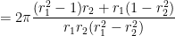
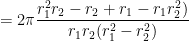








![\displaystyle \frac{2(1+[ir_1]^2)}{4 [ir_1]^3 + 2(4b^2-2) [ir_1]} = \displaystyle \frac{-i(1-r_1^2)}{-2r_1^3 + (4b^2-2) r_1}](https://s0.wp.com/latex.php?latex=%5Cdisplaystyle+%5Cfrac%7B2%281%2B%5Bir_1%5D%5E2%29%7D%7B4+%5Bir_1%5D%5E3+%2B+2%284b%5E2-2%29+%5Bir_1%5D%7D+%3D+%5Cdisplaystyle+%5Cfrac%7B-i%281-r_1%5E2%29%7D%7B-2r_1%5E3+%2B+%284b%5E2-2%29+r_1%7D&bg=ffffff&fg=000000&s=0&c=20201002)
![\displaystyle \frac{2(1+[ir_2]^2)}{4 [ir_2]^3 + 2(4b^2-2) [ir_2]} = \displaystyle \frac{-i(1-r_2^2)}{-2r_2^3 + (4b^2-2) r_2}](https://s0.wp.com/latex.php?latex=%5Cdisplaystyle+%5Cfrac%7B2%281%2B%5Bir_2%5D%5E2%29%7D%7B4+%5Bir_2%5D%5E3+%2B+2%284b%5E2-2%29+%5Bir_2%5D%7D+%3D+%5Cdisplaystyle+%5Cfrac%7B-i%281-r_2%5E2%29%7D%7B-2r_2%5E3+%2B+%284b%5E2-2%29+r_2%7D&bg=ffffff&fg=000000&s=0&c=20201002)
![Q = \displaystyle \lim_{R \to \infty} \oint_{C_R} \frac{ 2(1+z^2) dz}{z^4 + (4 b^2 - 2) z^2 + 1} = 2\pi i \left[\frac{-i(1-r_1^2)}{-2r_1^3 + (4b^2-2) r_1} +\frac{-i(1-r_2^2)}{-2r_2^3 + (4b^2-2) r_2} \right]](https://s0.wp.com/latex.php?latex=Q+%3D+%5Cdisplaystyle+%5Clim_%7BR+%5Cto+%5Cinfty%7D+%5Coint_%7BC_R%7D+%5Cfrac%7B+2%281%2Bz%5E2%29+dz%7D%7Bz%5E4+%2B+%284+b%5E2+-+2%29+z%5E2+%2B+1%7D+%3D+2%5Cpi+i+%5Cleft%5B%5Cfrac%7B-i%281-r_1%5E2%29%7D%7B-2r_1%5E3+%2B+%284b%5E2-2%29+r_1%7D+%2B%5Cfrac%7B-i%281-r_2%5E2%29%7D%7B-2r_2%5E3+%2B+%284b%5E2-2%29+r_2%7D+%5Cright%5D&bg=ffffff&fg=000000&s=0&c=20201002)





![Q'(a) = \displaystyle 2 \int_{-\infty}^{\infty} \frac{ 2a \left[ (a^2+b^2)^2 v^2 + b^2\right] - 2 (a^2+b^2) \cdot (a^2+b^2) v^2 \cdot 2a }{\left[ (a^2+b^2)^2 v^2 + b^2 \right]^2} dv](https://s0.wp.com/latex.php?latex=Q%27%28a%29+%3D+%5Cdisplaystyle+2+%5Cint_%7B-%5Cinfty%7D%5E%7B%5Cinfty%7D+%5Cfrac%7B+2a+%5Cleft%5B+%28a%5E2%2Bb%5E2%29%5E2+v%5E2+%2B+b%5E2%5Cright%5D+-+2+%28a%5E2%2Bb%5E2%29+%5Ccdot+%28a%5E2%2Bb%5E2%29+v%5E2+%5Ccdot+2a+%7D%7B%5Cleft%5B+%28a%5E2%2Bb%5E2%29%5E2+v%5E2+%2B+b%5E2+%5Cright%5D%5E2%7D+dv&bg=ffffff&fg=000000&s=0&c=20201002)
![Q'(a) = \displaystyle 4a \int_{-\infty}^{\infty} \frac{(a^2+b^2)^2 v^2 + b^2- 2 (a^2+b^2)^2 v^2}{\left[ (a^2+b^2)^2 v^2 + b^2 \right]^2} dv](https://s0.wp.com/latex.php?latex=Q%27%28a%29+%3D+%5Cdisplaystyle+4a+%5Cint_%7B-%5Cinfty%7D%5E%7B%5Cinfty%7D+%5Cfrac%7B%28a%5E2%2Bb%5E2%29%5E2+v%5E2+%2B+b%5E2-+2+%28a%5E2%2Bb%5E2%29%5E2+v%5E2%7D%7B%5Cleft%5B+%28a%5E2%2Bb%5E2%29%5E2+v%5E2+%2B+b%5E2+%5Cright%5D%5E2%7D+dv&bg=ffffff&fg=000000&s=0&c=20201002)
![Q'(a) = \displaystyle 4a \int_{-\infty}^{\infty} \frac{b^2-(a^2+b^2)^2 v^2}{\left[ (a^2+b^2)^2 v^2 + b^2 \right]^2} dv](https://s0.wp.com/latex.php?latex=Q%27%28a%29+%3D+%5Cdisplaystyle+4a+%5Cint_%7B-%5Cinfty%7D%5E%7B%5Cinfty%7D+%5Cfrac%7Bb%5E2-%28a%5E2%2Bb%5E2%29%5E2+v%5E2%7D%7B%5Cleft%5B+%28a%5E2%2Bb%5E2%29%5E2+v%5E2+%2B+b%5E2+%5Cright%5D%5E2%7D+dv&bg=ffffff&fg=000000&s=0&c=20201002)
![(a^2+b^2)^2 v^2 = (a^2+b^2)^2 \displaystyle \left[ \frac{b}{a^2+b^2} \tan \theta \right]^2 = b^2 \tan^2 \theta](https://s0.wp.com/latex.php?latex=%28a%5E2%2Bb%5E2%29%5E2+v%5E2+%3D+%28a%5E2%2Bb%5E2%29%5E2+%5Cdisplaystyle+%5Cleft%5B+%5Cfrac%7Bb%7D%7Ba%5E2%2Bb%5E2%7D+%5Ctan+%5Ctheta+%5Cright%5D%5E2+%3D+b%5E2+%5Ctan%5E2+%5Ctheta&bg=ffffff&fg=000000&s=0&c=20201002)
![Q'(a) = \displaystyle 4a \int_{-\pi/2}^{\pi/2} \frac{b^2- b^2 \tan^2 \theta}{\left[ b^2 \tan^2 \theta + b^2 \right]^2} \frac{b}{a^2+b^2} \sec^2 \theta \, d\theta](https://s0.wp.com/latex.php?latex=Q%27%28a%29+%3D+%5Cdisplaystyle+4a+%5Cint_%7B-%5Cpi%2F2%7D%5E%7B%5Cpi%2F2%7D+%5Cfrac%7Bb%5E2-+b%5E2+%5Ctan%5E2+%5Ctheta%7D%7B%5Cleft%5B+b%5E2+%5Ctan%5E2+%5Ctheta+%2B+b%5E2+%5Cright%5D%5E2%7D+%5Cfrac%7Bb%7D%7Ba%5E2%2Bb%5E2%7D+%5Csec%5E2+%5Ctheta+%5C%2C+d%5Ctheta&bg=ffffff&fg=000000&s=0&c=20201002)
![= \displaystyle \frac{4ab^3}{a^2+b^2} \int_{-\pi/2}^{\pi/2} \frac{[1- \tan^2 \theta] \sec^2 \theta}{\left[ \tan^2 \theta +1 \right]^2} d\theta](https://s0.wp.com/latex.php?latex=%3D+%5Cdisplaystyle+%5Cfrac%7B4ab%5E3%7D%7Ba%5E2%2Bb%5E2%7D+%5Cint_%7B-%5Cpi%2F2%7D%5E%7B%5Cpi%2F2%7D+%5Cfrac%7B%5B1-+%5Ctan%5E2+%5Ctheta%5D+%5Csec%5E2+%5Ctheta%7D%7B%5Cleft%5B+%5Ctan%5E2+%5Ctheta+%2B1+%5Cright%5D%5E2%7D+d%5Ctheta&bg=ffffff&fg=000000&s=0&c=20201002)
![= \displaystyle \frac{4ab^3}{a^2+b^2} \int_{-\pi/2}^{\pi/2} \frac{[1-\tan^2 \theta] \sec^2 \theta}{\left[ \sec^2 \theta \right]^2} d\theta](https://s0.wp.com/latex.php?latex=%3D+%5Cdisplaystyle+%5Cfrac%7B4ab%5E3%7D%7Ba%5E2%2Bb%5E2%7D+%5Cint_%7B-%5Cpi%2F2%7D%5E%7B%5Cpi%2F2%7D+%5Cfrac%7B%5B1-%5Ctan%5E2+%5Ctheta%5D+%5Csec%5E2+%5Ctheta%7D%7B%5Cleft%5B+%5Csec%5E2+%5Ctheta+%5Cright%5D%5E2%7D+d%5Ctheta&bg=ffffff&fg=000000&s=0&c=20201002)
![= \displaystyle \frac{4ab^3}{a^2+b^2} \int_{-\pi/2}^{\pi/2} \frac{[1-\tan^2 \theta] \sec^2 \theta}{\sec^4 \theta} d\theta](https://s0.wp.com/latex.php?latex=%3D+%5Cdisplaystyle+%5Cfrac%7B4ab%5E3%7D%7Ba%5E2%2Bb%5E2%7D+%5Cint_%7B-%5Cpi%2F2%7D%5E%7B%5Cpi%2F2%7D+%5Cfrac%7B%5B1-%5Ctan%5E2+%5Ctheta%5D+%5Csec%5E2+%5Ctheta%7D%7B%5Csec%5E4+%5Ctheta%7D+d%5Ctheta&bg=ffffff&fg=000000&s=0&c=20201002)
![= \displaystyle \frac{4ab^3}{a^2+b^2} \int_{-\pi/2}^{\pi/2} \frac{[1- \tan^2 \theta]}{\sec^2 \theta} d\theta](https://s0.wp.com/latex.php?latex=%3D+%5Cdisplaystyle+%5Cfrac%7B4ab%5E3%7D%7Ba%5E2%2Bb%5E2%7D+%5Cint_%7B-%5Cpi%2F2%7D%5E%7B%5Cpi%2F2%7D+%5Cfrac%7B%5B1-+%5Ctan%5E2+%5Ctheta%5D%7D%7B%5Csec%5E2+%5Ctheta%7D+d%5Ctheta&bg=ffffff&fg=000000&s=0&c=20201002)
![= \displaystyle \frac{4ab^3}{a^2+b^2} \int_{-\pi/2}^{\pi/2} [1- \tan^2 \theta] \cos^2 \theta \, d\theta](https://s0.wp.com/latex.php?latex=%3D+%5Cdisplaystyle+%5Cfrac%7B4ab%5E3%7D%7Ba%5E2%2Bb%5E2%7D+%5Cint_%7B-%5Cpi%2F2%7D%5E%7B%5Cpi%2F2%7D+%5B1-+%5Ctan%5E2+%5Ctheta%5D+%5Ccos%5E2+%5Ctheta+%5C%2C+d%5Ctheta&bg=ffffff&fg=000000&s=0&c=20201002)
![= \displaystyle \frac{4ab^3}{a^2+b^2} \int_{-\pi/2}^{\pi/2} [\cos^2 \theta -\sin^2 \theta] d\theta](https://s0.wp.com/latex.php?latex=%3D+%5Cdisplaystyle+%5Cfrac%7B4ab%5E3%7D%7Ba%5E2%2Bb%5E2%7D+%5Cint_%7B-%5Cpi%2F2%7D%5E%7B%5Cpi%2F2%7D+%5B%5Ccos%5E2+%5Ctheta+-%5Csin%5E2+%5Ctheta%5D+d%5Ctheta&bg=ffffff&fg=000000&s=0&c=20201002)

![= \displaystyle \left[ \frac{2ab^3}{a^2+b^2} \sin 2\theta \right]^{\pi/2}_{-\pi/2}](https://s0.wp.com/latex.php?latex=%3D+%5Cdisplaystyle+%5Cleft%5B+%5Cfrac%7B2ab%5E3%7D%7Ba%5E2%2Bb%5E2%7D+%5Csin+2%5Ctheta+%5Cright%5D%5E%7B%5Cpi%2F2%7D_%7B-%5Cpi%2F2%7D&bg=ffffff&fg=000000&s=0&c=20201002)
![= \displaystyle \frac{2ab^3}{a^2+b^2} \left[ \sin \pi - \sin (-\pi) \right]](https://s0.wp.com/latex.php?latex=%3D+%5Cdisplaystyle+%5Cfrac%7B2ab%5E3%7D%7Ba%5E2%2Bb%5E2%7D+%5Cleft%5B+%5Csin+%5Cpi+-+%5Csin+%28-%5Cpi%29+%5Cright%5D&bg=ffffff&fg=000000&s=0&c=20201002)
![= \displaystyle \frac{2ab^3}{a^2+b^2} \left[ 0- 0 \right]](https://s0.wp.com/latex.php?latex=%3D+%5Cdisplaystyle+%5Cfrac%7B2ab%5E3%7D%7Ba%5E2%2Bb%5E2%7D+%5Cleft%5B+0-+0+%5Cright%5D&bg=ffffff&fg=000000&s=0&c=20201002)



![= \displaystyle \lim_{h \to 0} \left[ n x^{n-1} + \frac{1}{2} n(n-1) x^{n-2} h + \dots + h^{n-1} \right]](https://s0.wp.com/latex.php?latex=%3D+%5Cdisplaystyle+%5Clim_%7Bh+%5Cto+0%7D+%5Cleft%5B+n+x%5E%7Bn-1%7D+%2B+%5Cfrac%7B1%7D%7B2%7D+n%28n-1%29+x%5E%7Bn-2%7D+h+%2B+%5Cdots+%2B+h%5E%7Bn-1%7D+%5Cright%5D&bg=ffffff&fg=000000&s=0&c=20201002)




![y^q = \displaystyle \left[ x^{p/q} \right]^q](https://s0.wp.com/latex.php?latex=y%5Eq+%3D+%5Cdisplaystyle+%5Cleft%5B+x%5E%7Bp%2Fq%7D+%5Cright%5D%5Eq&bg=ffffff&fg=000000&s=0&c=20201002)


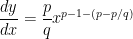
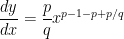
![\displaystyle \frac{dy}{dx} = \displaystyle \frac{p}{q} \frac{x^{p-1}}{[x^{p/q}]^{q-1}}](https://s0.wp.com/latex.php?latex=%5Cdisplaystyle+%5Cfrac%7Bdy%7D%7Bdx%7D+%3D+%5Cdisplaystyle+%5Cfrac%7Bp%7D%7Bq%7D+%5Cfrac%7Bx%5E%7Bp-1%7D%7D%7B%5Bx%5E%7Bp%2Fq%7D%5D%5E%7Bq-1%7D%7D&bg=ffffff&fg=000000&s=0&c=20201002)