In my capstone class for future secondary math teachers, I ask my students to come up with ideas for engaging their students with different topics in the secondary mathematics curriculum. In other words, the point of the assignment was not to devise a full-blown lesson plan on this topic. Instead, I asked my students to think about three different ways of getting their students interested in the topic in the first place.
I plan to share some of the best of these ideas on this blog (after asking my students’ permission, of course).
This student submission comes from my former student Shama Surani. Her topic, from Precalculus: using right-triangle trigonometry.

How could you as a teacher create an activity or project that involves your topic?

A project that Dorathy Scrudder, Sam Smith, and I did that involves right-triangle trigonometry in our PBI class last week, was to have the students to build bridges. Our driving question was “How can we redesign the bridge connecting I-35 and 635?” The students knew that the hypotenuse would be 34 feet, because there were two lanes, twelve feet each, and a shoulder of ten feet that we provided on a worksheet. As a group, they needed to decide on three to four angles between 10-45 degrees, and calculate the sine and cosine of the angle they chose. One particular group used the angle measures of 10°, 20°, 30°, and 40°. They all calculated the sine of their angles to find the height of the triangle, and used cosine to find the width of their triangle by using 34 as their hypotenuse. The picture above is by Sam Smith, and it illustrates the triangles that we wanted the students to calculate.
The students were instructed to make a scale model of a bridge so they were told that 1 feet = 0.5 centimeters. Hence, the students had to divide all their calculations by two. Then, the students had to check their measurements of their group members, and were provided materials such as cardstock, scissors, pipe cleaners, tape, rulers, and protractors in order to construct their bridges. They had to use a ruler to measure out what they found for sine and cosine on the cardstock, and make sure when they connected the line to make the hypotenuse that the hypotenuse had a length of 17 centimeters. After they drew their triangles, they had to use a protractor to verify that the angle they chose is what one of the angles were in the triangle. When our students presented, they were able to communicate what sine and cosine represented, and grasped the concepts.
Below are pictures of the triangles and bridges that one of our groups of students constructed. Overall, the students enjoyed this project, and with some tweaks, I believe this will be an engaging project for right triangle trigonometry.


How does this topic extend what your students should have learned in previous courses?
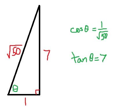
In previous classes, such in geometry, students should have learned about similar and congruent triangles in addition to triangle congruence such as side-side-side and side-angle-side. They should also have learned if they have a right angle triangle, and they are given two sides, they can find the other side by using the Pythagorean Theorem. The students should also have been exposed to special right triangles such as the 45°-45°-90° triangles and 30°-60°-90° triangles and the relationships to the sides. Right triangle trigonometry extends the ideas of these previous classes. Students know that there must be a 45°-45°-90° triangle has side lengths of 1, 1, and  which the lengths of 1 subtending the 45° angles. They also are aware that a 30°-60°-90° produces side lengths of 1,
  , and 2, with the side length of 1 subtending the 30°, the length of subtending the angle of 60°, and the length of 2 subtending the right angle. So, what happens when there is a right angle triangle, but the other two angles are not 45 degrees or 30 and 60 degrees? This is where right triangle trigonometry comes into play. Students will now be able to calculate the sine, cosine, and tangent and its reciprocal functions for those triangles that are right. Later, this topic will be extended to the unit circle and graphing the trigonometric functions as well as their reciprocal functions and inverse functions.
What are the contributions of various cultures to this topic?
Below are brief descriptions of various cultures that personally interested me.
Early Trigonometry
The Babylonians and Egyptians studied the sides of triangles other than angle measure since the concept of angle measure was not yet discovered. The Babylonian astronomers had detailed records on the rising and setting of stars, the motion of planets, and the solar and lunar eclipses. On the other hand, Egyptians used a primitive form of trigonometry in order to build the pyramids.
Greek Mathematics
Hipparchus of Nicaea, now known as the father of Trigonometry, compiled the first trigonometric table. He was the first one to formulate the corresponding values of arc and chord for a series of angles. Claudius Ptolemy wrote Almagest, which expanded on the ideas of Hipparchus’ ideas of chords in a circle. The Almagest is about astronomy, and astronomy relies heavily on trigonometry.
Indian Mathematics
Influential works called Siddhantas from the 4th-5th centry, first defined sine as the modern relationship between half an angle and half a chord. It also defined cosine, versine (which is 1 – cosine), and inverse sine. Aryabhata, an Indian astronomer and mathematician, expanded on the ideas of Siddhantas in another important work known as Aryabhatiya. Both of these works contain the earliest surviving tables of sine and versine values from 0 to 90 degrees, accurate to 4 decimal places. Interestingly enough, the words jya was for sine and kojya for cosine. It is now known as sine and cosine due to a mistranslation.
Islamic Mathematics
Muhammad ibn Mūsā al-Khwārizmī had produced accurate sine and cosine tables in the 9th century AD. Habash al-Hasib al-Marwazi was the first to produce the table of cotangents in 830 AD. Similarly, Muhammad ibn Jābir al-Harrānī al-Battānī had discovered the reciprocal functions of secant and cosecant. He also produced the first table of cosecants.
Muslim mathematicians were using all six trigonometric functions by the 10th century. In fact, they developed the method of triangulation which helped out with geography and surveying.
Chinese Mathematics
In China, early forms of trigonometry were not as widely appreciated as it was with the Greeks, Indians, and Muslims. However, Chinese mathematicians needed spherical geometry for calendrical science and astronomical calculations. Guo Shoujing improved the calendar system and Chinese astronomy by using spherical trigonometry in his calculations.
European Mathematics
Regiomontanus treated trigonometry as a distinct mathematical discipline. A student of Copernicus, Georg Joachim Rheticus, was the first one to define all six trigonometric functions in terms of right triangles other than circles in Opus palatinum de triangulis. Valentin Otho finished his work in 1596.
http://en.wikipedia.org/wiki/History_of_trigonometry


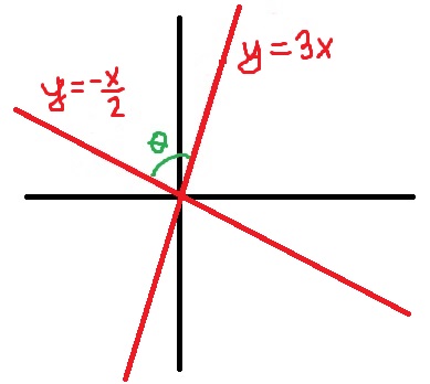
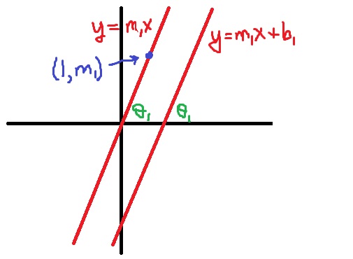 The lines


 and
and  .
.
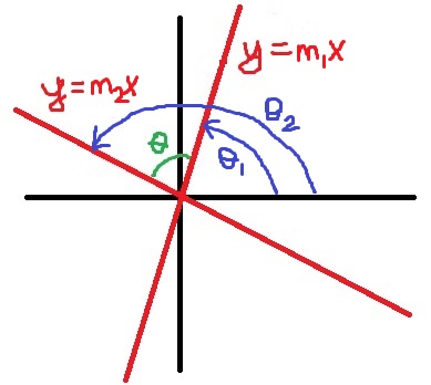
 and
and  . I use the caveat almost because the angle between two vectors could be between
  , while the smallest angle between two lines must lie between
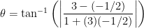


 .
. .
.
 and
and  . To begin, we draw the vectors
  (to be determined momentarily) that connects the tips of the vectors
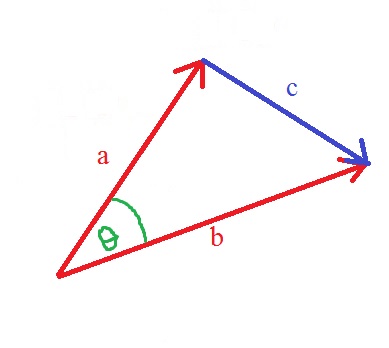
 , so that


 , convert the square of the norms into dot products. We then use the distributive and commutative properties of dot products to simplify.


 :
:
 and
and  ). Since this is the range of arccosine, we are permitted to use this inverse function to solve for
 for any dimension
  .
.
 and
and 
 is the dot product (or inner product) of the two vectors
  is the norm (or length) of the vector

 if
if  ,
,  , and
, and  .
. :
:


 :
:

 or if
or if  .
.


 (pretending that we didn’t do the work above). Let’s solve for

![[0^\circ, 180^\circ]](https://s0.wp.com/latex.php?latex=%5B0%5E%5Ccirc%2C+180%5E%5Ccirc%5D&bg=ffffff&fg=000000&s=0&c=20201002) , namely,
, namely,  and
and  . However, we know full well that the answer can’t be larger than
  .
. latex a = 16$,
  .
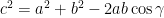
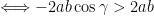
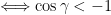
. , thus quickly demonstrating that the triangle is impossible. However, this also falls out of the Law of Cosines:


 ,
,  , and
, and  are all positive)

 . And the good news is that there is no need to overthink this… this is guaranteed to be the angle since the range of
  is
is ![[0,\pi]](https://s0.wp.com/latex.php?latex=%5B0%2C%5Cpi%5D&bg=ffffff&fg=000000&s=0&c=20201002) , or
, or 
 . And since an angle in a triangle must lie between
 ![[0^\circ,90^\circ]](https://s0.wp.com/latex.php?latex=%5B0%5E%5Ccirc%2C90%5E%5Ccirc%5D&bg=ffffff&fg=000000&s=0&c=20201002) and also the interval
and also the interval ![[90^\circ, 180^\circ]](https://s0.wp.com/latex.php?latex=%5B90%5E%5Ccirc%2C+180%5E%5Ccirc%5D&bg=ffffff&fg=000000&s=0&c=20201002) .
. :
: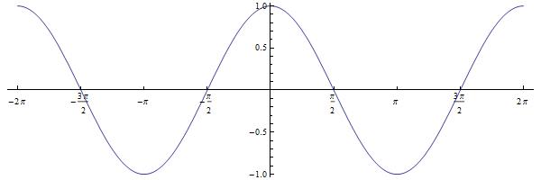
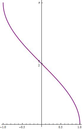
 , we select a section that satisfies the horizontal line test and ignore the rest of the graph. (I described this in more rigorous terms when I considered arcsine, so I will not repeat the rigor here.) There are plenty of choices that could be made; by tradition, the interval
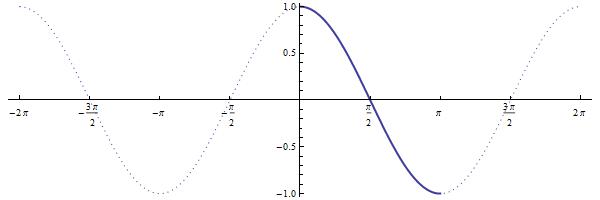
 produces the graph of
  . Again, to assist my students when graphing this function, I point out that the graph of cosine has horizontal tangent lines at the points
  and
and  . Therefore, after reflecting through the line
  has vertical tangent lines at
  and
and  .
.
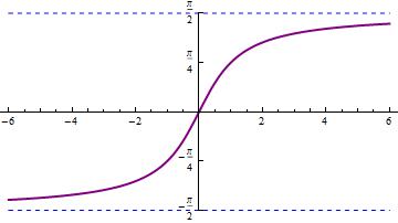
 is chosen as the section of the graph of
  that satisfies the horizontal line test.
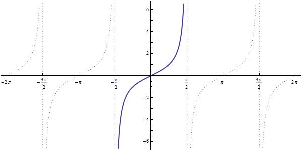
 . Like the (more complicated)
  .
.
 means that
  and
and 
 and
and 


 . This of course is commonly called the distributive property (and not the commutative property), but the essential idea is that the same answer is obtained whether the multiplications are performed first or if the addition is performed first.
 , then
  .
. is any real number, then
  .
. .
. .
. is continuous at an interior point
  .
. are differentiable, then
  .
. .
. .
. .
. is integrable,
  .
. .
. and
and  are random variables, then
  .
. .
. .
. .
. ,
,  , and
, and  are sets, then
  .
. .
. if
if  . Important special cases are
  ,
,  , and
, and  .
. . I call this the
  .
. ,
,  , etc.
 .
. .
.
 .
. .
. .
.