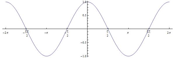
In this series, we’ve seen that the inverse of function that fails the horizontal line test can be defined by appropriately restricting the domain of the function. For example, we now look at the graph of :

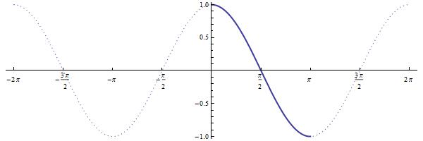
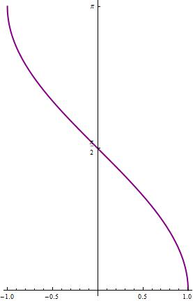
As with the graph of , we select a section that satisfies the horizontal line test and ignore the rest of the graph. (I described this in more rigorous terms when I considered arcsine, so I will not repeat the rigor here.) There are plenty of choices that could be made; by tradition, the interval is chosen.

Reflecting only the half-wave of the cosine graph on the interval through the line produces the graph of . Again, to assist my students when graphing this function, I point out that the graph of cosine has horizontal tangent lines at the points and . Therefore, after reflecting through the line , we see that the graph of has vertical tangent lines at and .

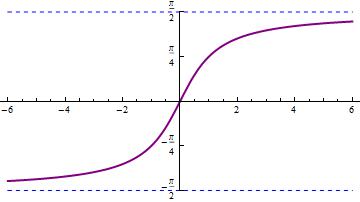
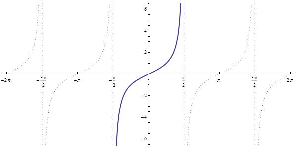
The same logic applies when defining the arctangent function. By tradition, the interval is chosen as the section of the graph of that satisfies the horizontal line test.

Reflecting only the half-wave of the cosine graph on the interval through the line produces the graph of . Like the (more complicated) logistic growth function, this function has two different horizontal asymptotes that govern the behavior of the function as .

So here are the rules that I want my Precalculus students to memorize:

means that and

means that and

means that and

Students using forget that the range of arccosine is different than the other two, and I’ll usually have to produce the graph of to explain and re-explain why this one is different.

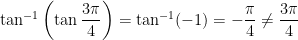
Because these functions are defined on restricted domains, the usual funny things can happen. For example,