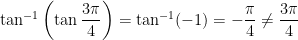
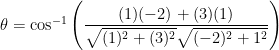
Arccosine has an important advantage over arcsine when solving for the parts of a triangle: there is no possibility ambiguity about the angle.
Solve  if
if  ,
,  , and
, and  .
.
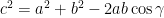
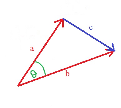
When solving for the three angles, it’s best to start with the biggest angle (that is, the angle opposite the biggest side). To see why, let’s see what happens if we first use the Law of Cosines to solve for one of the two smaller angles, say  :
:


So far, so good. Now let’s try using the Law of Sines to solve for  :
:


Uh oh… there are two possible solutions for since, hypothetically, could be in either the first or second quadrant! So we have no way of knowing, using only the Law of Sines, whether  or if
or if  .
.
 For this reason, it would have been far better to solve for the biggest angle first. For the present example, the biggest answer is since that’s the angle opposite the longest side.


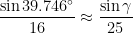
Using a calculator, we find that .
We now use the Law of Sines to solve for either or  (pretending that we didn’t do the work above). Let’s solve for :


This equation also has two solutions in the interval ![[0^\circ, 180^\circ]](https://s0.wp.com/latex.php?latex=%5B0%5E%5Ccirc%2C+180%5E%5Ccirc%5D&bg=ffffff&fg=000000&s=0&c=20201002) , namely,
, namely,  and
and  . However, we know full well that the answer can’t be larger than since that’s already known to be the largest angle. So there’s no need to overthink the matter — the answer from blindly using arcsine on a calculator is going to be the answer for .
Naturally, the easiest way of finding is by computing  .
.


 Using the usual rules for adding vectors, we see that


 and
and  .
.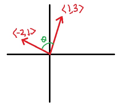
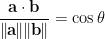
 and
and  . The angle
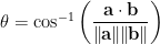
 is the dot product (or inner product) of the two vectors
  is the norm (or length) of the vector
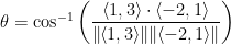


 latex a = 16$,
  .
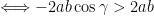
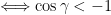
. , thus quickly demonstrating that the triangle is impossible. However, this also falls out of the Law of Cosines:


 ,
,  , and
, and  are all positive)

 . And the good news is that there is no need to overthink this… this is guaranteed to be the angle since the range of
  is
is ![[0,\pi]](https://s0.wp.com/latex.php?latex=%5B0%2C%5Cpi%5D&bg=ffffff&fg=000000&s=0&c=20201002) , or
, or 
 . And since an angle in a triangle must lie between
 ![[0^\circ,90^\circ]](https://s0.wp.com/latex.php?latex=%5B0%5E%5Ccirc%2C90%5E%5Ccirc%5D&bg=ffffff&fg=000000&s=0&c=20201002) and also the interval
and also the interval ![[90^\circ, 180^\circ]](https://s0.wp.com/latex.php?latex=%5B90%5E%5Ccirc%2C+180%5E%5Ccirc%5D&bg=ffffff&fg=000000&s=0&c=20201002) .
. :
: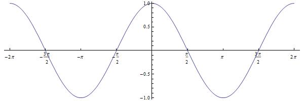
 , we select a section that satisfies the horizontal line test and ignore the rest of the graph. (I described this in more rigorous terms when I considered arcsine, so I will not repeat the rigor here.) There are plenty of choices that could be made; by tradition, the interval
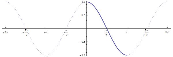
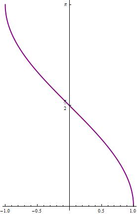
 produces the graph of
  . Again, to assist my students when graphing this function, I point out that the graph of cosine has horizontal tangent lines at the points
  and
and  . Therefore, after reflecting through the line
  has vertical tangent lines at
  and
and  .
.
 is chosen as the section of the graph of
  that satisfies the horizontal line test.
 . Like the (more complicated)
  .
.
 means that
  and
and 
 and
and