Every once in a while, I’ll give a “fun lecture” to my students. The rules of a “fun lecture” are that I talk about some advanced applications of classroom topics, but I won’t hold them responsible for these ideas on homework and on exams. In other words, they can just enjoy the lecture without being responsible for its content.
In this series of posts, I’m describing a fun lecture on generating functions that I’ve given to my Precalculus students. In the previous post, we looked at the famed Fibonacci sequence

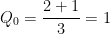
We also looked at that (slightly less famous) Quintanilla sequence

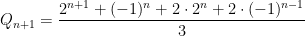
which is defined so that each term is the sum of the previous term and twice the term that’s two back in the sequence. Using the concept of a generating function, we found that the 


To close out the fun lecture, I’ll then verify that this formula works by using mathematical induction. As seen below, it’s a lot less work to verify the formula with mathematical induction than to derive it from the generating function.


That’s the formula if
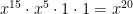
Let me note parenthetically that the above simplification is not all intuitive when encountered by students for the first time — even really bright students who know the laws of exponents cold and who know full well that 


By this point, I’m usually near the end of my 50-minute fun lecture. Since students are not responsible for replicating the contents of the fun lecture, I’ve found that most students are completely comfortable with this pace of presentation.
Then I ask my students which way they’d prefer: generating functions or mathematical induction? They usually respond induction. However, they also are able to realize that the thing that makes mathematical induction is also the challenge: they have to guess the correct formula and then use induction to verify that the formula actually works. On the other hand, with generating functions, there’s no need to guess the correct answer… you just follow the steps and see what comes out the other side.
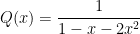
Finally, to close the fun lecture, I tell them that the above steps can be used to find a closed-form expression for the Fibonacci sequence. (I devised the Quintanilla sequence for pedagogical purposes: since the denominator of its generating function easily factors, the subsequent steps aren’t too messy.) I won’t go through all the steps here, so I’ll leave it as a challenge for the reader to start with the generating function

factor the denominator by finding the two real roots of 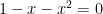
I conclude this post with some pedagogical reflections. I taught this fun lecture to about 10 different Precalculus classes, and it was a big hit each time. I think that my students were thoroughly engaged with the topic and liked seeing an unorthodox application of the various topics in Precalculus that they were learning (sequences, series, partial fractions, factoring polynomials over 
I covered the content of this series of five posts in a 50-minute lecture. I’d usually finish the proof by induction as time expired and then would challenge them to think about how to similarly find the formula for the Fibonacci sequence. The rules of a “fun lecture” were important to pull this off — I made it clear that students would not have to do this for homework, so the pressure was off them to understand the fine details during the lecture. Instead, the idea was for them to appreciate the big picture of how topics in Precalculus can be used in future courses.
 . Notice that the denominator factors easily, so that
 and
and  so that
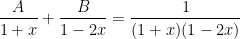 ,
,
 .
. , then we obtain
  , or
, or  .
. , then we obtain
  , or
, or  .
.

 term is
 ,
, term is
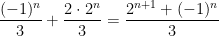
 , which was obtained without knowing the 10th and 11th terms.
 s, and each subsequent term is defined as the sum of the two previous terms. Of course, the generating function for this sequence is


 to get the answer.
 and
and  and also
  :
:

![[1 - x - 2x^2] Q(x) = 1](https://s0.wp.com/latex.php?latex=%5B1+-+x+-+2x%5E2%5D+Q%28x%29+%3D+1&bg=ffffff&fg=000000&s=0&c=20201002)
![\left[1 + x + x^2 + x^3 + x^4 + x^5 + \dots \right]](https://s0.wp.com/latex.php?latex=%5Cleft%5B1+%2B+x+%2B+x%5E2+%2B+x%5E3+%2B+x%5E4+%2B+x%5E5+%2B+%5Cdots+%5Cright%5D&bg=ffffff&fg=000000&s=0&c=20201002)
![\times \left[1 + x^5 + x^{10} + x^{15} + x^{20} + x^{25} + \dots \right]](https://s0.wp.com/latex.php?latex=%5Ctimes+%5Cleft%5B1+%2B+x%5E5+%2B+x%5E%7B10%7D+%2B+x%5E%7B15%7D+%2B+x%5E%7B20%7D+%2B+x%5E%7B25%7D+%2B+%5Cdots+%5Cright%5D&bg=ffffff&fg=000000&s=0&c=20201002)
![\times \left[1 + x^{10} + x^{20} + x^{30} + x^{40} + x^{50} + \dots \right]](https://s0.wp.com/latex.php?latex=%5Ctimes+%5Cleft%5B1+%2B+x%5E%7B10%7D+%2B+x%5E%7B20%7D+%2B+x%5E%7B30%7D+%2B+x%5E%7B40%7D+%2B+x%5E%7B50%7D+%2B+%5Cdots+%5Cright%5D&bg=ffffff&fg=000000&s=0&c=20201002)
![\times \left[1 + x^{25} + x^{50} + x^{75} + x^{100} + x^{125} + \dots \right]](https://s0.wp.com/latex.php?latex=%5Ctimes+%5Cleft%5B1+%2B+x%5E%7B25%7D+%2B+x%5E%7B50%7D+%2B+x%5E%7B75%7D+%2B+x%5E%7B100%7D+%2B+x%5E%7B125%7D+%2B+%5Cdots+%5Cright%5D&bg=ffffff&fg=000000&s=0&c=20201002)
 from the product of these four infinite series? I offer a thought bubble if you’d like to think about it before seeing the answer.


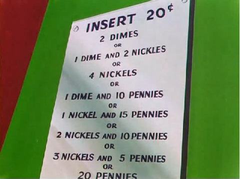
 : 15 pennies (15 cents) and 1 nickel (5 cents)
 ), we may write the infinite product as
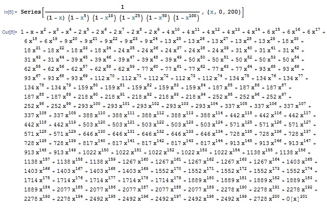
 — the coefficients provide the number of ways of expressing that many cents using pennies, nickels, dimes and quarters. This Taylor series can be computed with Mathematica:
 . The generating function for this sequence is
 , using the formula for an infinite geometric series.
 , the generating function is
 ,
, .
. if $0 \le n \le 10$ and
  for
for  . Then the generating function is
 .
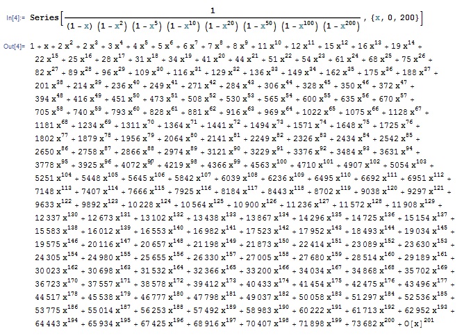
. denote the number of ways that
  . What about one dollar? Two dollars? I’ll provide the answer in tomorrow’s post.
 or
or  ? From example, here’s a simple problem from trigonometry:
 is an acute angle so that
  . Find
  .
.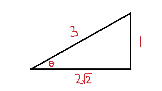
 . The adjacent side has length
 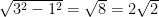 . Therefore,

 or
or  to nine decimal places? Clearly, the first step is finding
  by hand,
  or
or 
 or divide by
  ?
? . The inductive step showed that since the rule is valid for
  , which in turn implies that the rule is valid for
  and so on.

![[a_2, -a_1]^T](https://s0.wp.com/latex.php?latex=%5Ba_2%2C+-a_1%5D%5ET&bg=ffffff&fg=000000&s=0&c=20201002) … the matrix is an example of a rotation matrix. This concept appears quite frequently in linear algebra (not to mention video games and computer graphics). In the secondary mathematics curriculum, this device is often used to determine how to graph conic sections of the form
… the matrix is an example of a rotation matrix. This concept appears quite frequently in linear algebra (not to mention video games and computer graphics). In the secondary mathematics curriculum, this device is often used to determine how to graph conic sections of the form ,
, . I’ll refer to the