I’m pleased to say that my latest paper, “A New Derivation of Snell’s Law without Calculus,” has now been published in College Mathematics Journal. The article is now available for online access to anyone who has access to the journal — usually, that means members of the Mathematical Association of America or anyone whose employer (say, a university) has institutional access. I expect that it will be in the printed edition of the journal later this year; however, I’ve not been told yet the issue in which it will appear.
Because of copyright issues, I can’t reproduce my new derivation of Snell’s Law here on the blog, so let me instead summarize the main idea. Snell’s Law (see Wikipedia) dictates the angle at which light is refracted when it passes from one medium (say, air) into another (say, water). If the velocity of light through air is while its velocity in water is , then Snell’s Law says that
From Wikipedia
I was asked by a bright student who was learning physics if there was a way to prove Snell’s Law without using calculus. At the time, I was blissfully unaware of Huygens’s Principle (see OpenStax) and I didn’t have a good answer. I had only seen derivations of Snell’s Law using the first-derivative test, which is a standard optimization problem found in most calculus books (again, see Wikipedia) based on Fermat’s Principle that light travels along a path that minimizes time.
Anyway, after a couple of days, I found an elementary proof that does not require proof. I should warn that the word “elementary” can be a loaded word when used by mathematicians. The proof uses only concepts found in Precalculus, especially rotating a certain hyperbola and careful examining the domain of two functions. So while the proof does not use calculus, I can’t say that the proof is particularly easy — especially compared to the classical proof using Huygens’s Principle.
That said, I’m pretty sure that my proof is original, and I’m pretty proud of it.
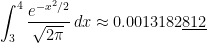
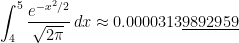
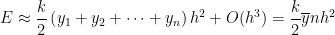
I end this series about numerical integration by returning to the most common (if hidden) application of numerical integration in the secondary mathematics curriculum: finding the area under the normal curve. This is a critically important tool for problems in both probability and statistics; however, the antiderivative of cannot be expressed using finitely many elementary functions. Therefore, we must resort to numerical methods instead.
In days of old, of course, students relied on tables in the back of the textbook to find areas under the bell curve, and I suppose that such tables are still being printed. For students with access to modern scientific calculators, of course, there’s no need for tables because this is a built-in function on many calculators. For the line of TI calculators, the command is normalcdf.
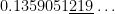
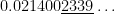
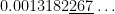
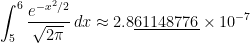
Unfortunately, it’s a sad (but not well-known) fact of life that the TI-83 and TI-84 calculators are not terribly accurate at computing these areas. For example:
TI-84:
Correct answer, with Mathematica:
TI-84:
Correct answer, with Mathematica:
TI-84:
Correct answer, with Mathematica:
TI-84:
Correct answer, with Mathematica:
TI-84:
Correct answer, with Mathematica:
TI-84:
Correct answer, with Mathematica:
I don’t presume to know the proprietary algorithm used to implement normalcdf on TI-83 and TI-84 calculators. My honest if brutal assessment is that it’s probably not worth knowing: in the best case (when the endpoints are close to 0), the calculator provides an answer that is accurate to only 7 significant digits while presenting the illusion of a higher degree of accuracy. I can say that Simpson’s Rule with only subintervals provides a better approximation to than the normalcdf function.
For what it’s worth, I also looked at the accuracy of the NORMSDIST function in Microsoft Excel. This is much better, almost always producing answers that are accurate to 11 or 12 significant digits, which is all that can be realistically expected in floating-point double-precision arithmetic (in which numbers are usually stored accurate to 13 significant digits prior to any computations).
Numerical integration is a standard topic in first-semester calculus. From time to time, I have received questions from students on various aspects of this topic, including:
Why is numerical integration necessary in the first place?
Where do these formulas come from (especially Simpson’s Rule)?
How can I do all of these formulas quickly?
Is there a reason why the Midpoint Rule is better than the Trapezoid Rule?
Is there a reason why both the Midpoint Rule and the Trapezoid Rule converge quadratically?
Is there a reason why Simpson’s Rule converges like the fourth power of the number of subintervals?
In this series, I hope to answer these questions. While these are standard questions in a introductory college course in numerical analysis, and full and rigorous proofs can be found on Wikipedia and Mathworld, I will approach these questions from the point of view of a bright student who is currently enrolled in calculus and hasn’t yet taken real analysis or numerical analysis.
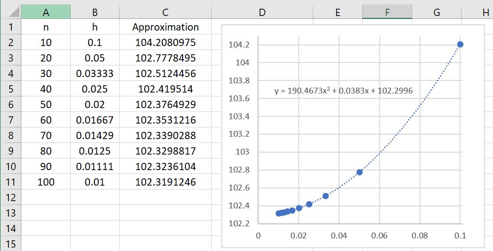
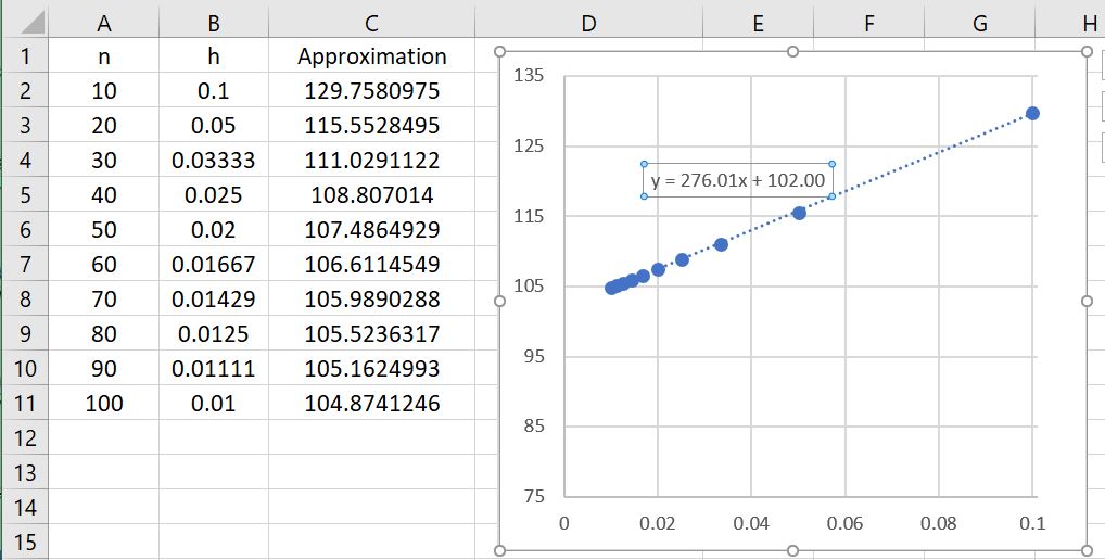
In this series, we have shown the following approximations of errors when using various numerical approximations for . We obtained these approximations using only techniques within the reach of a talented high school student who has mastered Precalculus — especially the Binomial Theorem — and elementary techniques of integration.
As we now present, the formulas that we derived are (of course) easily connected to known theorems for the convergence of these techniques. These proofs, however, require some fairly advanced techniques from calculus. So, while the formulas derived in this series of posts only apply to (and, by an easy extension, any polynomial), the formulas that we do obtain easily foreshadow the actual formulas found on Wikipedia or Mathworld or calculus textbooks, thus (hopefully) taking some of the mystery out of these formulas.
Numerical integration is a standard topic in first-semester calculus. From time to time, I have received questions from students on various aspects of this topic, including:
Why is numerical integration necessary in the first place?
Where do these formulas come from (especially Simpson’s Rule)?
How can I do all of these formulas quickly?
Is there a reason why the Midpoint Rule is better than the Trapezoid Rule?
Is there a reason why both the Midpoint Rule and the Trapezoid Rule converge quadratically?
Is there a reason why Simpson’s Rule converges like the fourth power of the number of subintervals?
In this series, I hope to answer these questions. While these are standard questions in a introductory college course in numerical analysis, and full and rigorous proofs can be found on Wikipedia and Mathworld, I will approach these questions from the point of view of a bright student who is currently enrolled in calculus and hasn’t yet taken real analysis or numerical analysis.
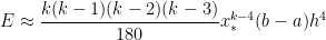
In this previous post in this series, we showed that the Simpson’s Rule approximation of has an error of
.
In this post, we consider the global error when integrating on the interval instead of a subinterval .
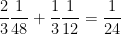
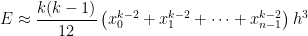
The total error when approximating will be the sum of the errors for the integrals over , , through . Therefore, the total error will be
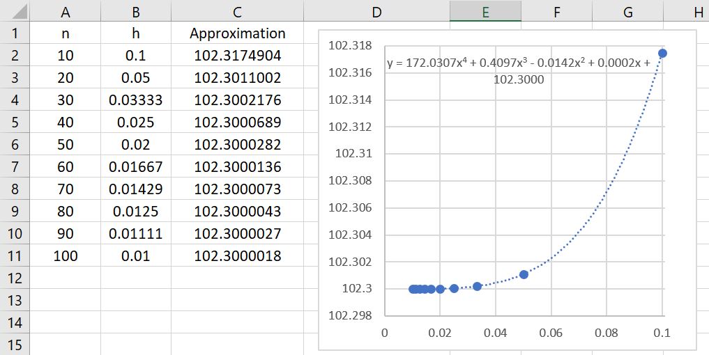
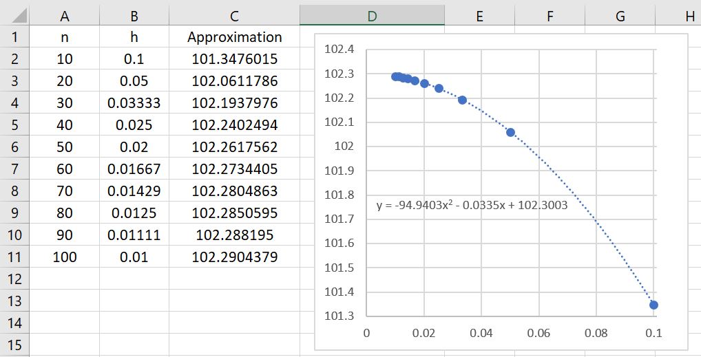
So that this formula doesn’t appear completely mystical, this actually matches the numerical observations that we made earlier. The figure below shows the left-endpoint approximations to for different numbers of subintervals. If we take and , then the error should be approximately equal to
,
which, as expected, is close to the observed error of .
Let , so that the error becomes
,
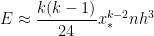
where is the average of the . (We notice that there are only terms in this sum since we’re adding only the even terms.) Clearly, this average is somewhere between the smallest and the largest of the . Since is a continuous function, that means that there must be some value of between and — and therefore between and — so that by the Intermediate Value Theorem. We conclude that the error can be written as
,
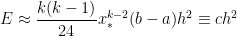
Finally, since is the length of one subinterval, we see that is the total length of the interval . Therefore,
,
where the constant is determined by , , and . In other words, for the special case , we have established that the error from Simpson’s Rule is approximately quartic in — without resorting to the generalized mean-value theorem and confirming the numerical observations we made earlier.
Numerical integration is a standard topic in first-semester calculus. From time to time, I have received questions from students on various aspects of this topic, including:
Why is numerical integration necessary in the first place?
Where do these formulas come from (especially Simpson’s Rule)?
How can I do all of these formulas quickly?
Is there a reason why the Midpoint Rule is better than the Trapezoid Rule?
Is there a reason why both the Midpoint Rule and the Trapezoid Rule converge quadratically?
Is there a reason why Simpson’s Rule converges like the fourth power of the number of subintervals?
In this series, I hope to answer these questions. While these are standard questions in a introductory college course in numerical analysis, and full and rigorous proofs can be found on Wikipedia and Mathworld, I will approach these questions from the point of view of a bright student who is currently enrolled in calculus and hasn’t yet taken real analysis or numerical analysis.
In this post, we will perform an error analysis for Simpson’s Rule
where is the number of subintervals (which has to be even) and is the width of each subinterval, so that .
As noted above, a true exploration of error analysis requires the generalized mean-value theorem, which perhaps a bit much for a talented high school student learning about this technique for the first time. That said, the ideas behind the proof are accessible to high school students, using only ideas from the secondary curriculum (especially the Binomial Theorem), if we restrict our attention to the special case , where is a positive integer.
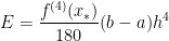
For this special case, the true area under the curve on the subinterval will be
In the above, the shorthand can be formally defined, but here we’ll just take it to mean “terms that have a factor of or higher that we’re too lazy to write out.” Since is supposed to be a small number, these terms will small in magnitude and thus can be safely ignored.
Earlier in this series, we derived the very convenient relationship relating the approximations from Simpson’s Rule, the Midpoint Rule, and the Trapezoid Rule. We now exploit this relationship to approximate . Earlier in this series, we found the Midpoint Rule approximation on this subinterval to be
while we found the Trapezoid Rule approximation to be
.
Therefore, if there are subintervals, the Simpson’s Rule approximation of — that is, the area under the parabola that passes through , , and — will be . Since
,
,
and
,
we see that
.
We notice that something wonderful just happened: the first four terms of perfectly match the first four terms of the exact value of the integral! Subtracting from the actual integral, the error in this approximation will be equal to
Before moving on, there’s one minor bookkeeping issue to deal with. We note that this is the error for , where subintervals are used. However, the value of in this equal arose from and , where only subintervals are used. So let’s write the error with subintervals as
,
where is the width of all of the subintervals. By analogy, we see that the error for subintervals will be
.
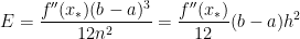
But even after adjusting for this constant, we see that this local error behaves like , a vast improvement over both the Midpoint Rule and the Trapezoid Rule. This illustrates a general principle of numerical analysis: given two algorithms that are , an improved algorithm can typically be made by taking some linear combination of the two algorithms. Usually, the improvement will be to ; however, in this example, we magically obtained an improvement to .
Numerical integration is a standard topic in first-semester calculus. From time to time, I have received questions from students on various aspects of this topic, including:
Why is numerical integration necessary in the first place?
Where do these formulas come from (especially Simpson’s Rule)?
How can I do all of these formulas quickly?
Is there a reason why the Midpoint Rule is better than the Trapezoid Rule?
Is there a reason why both the Midpoint Rule and the Trapezoid Rule converge quadratically?
Is there a reason why Simpson’s Rule converges like the fourth power of the number of subintervals?
In this series, I hope to answer these questions. While these are standard questions in a introductory college course in numerical analysis, and full and rigorous proofs can be found on Wikipedia and Mathworld, I will approach these questions from the point of view of a bright student who is currently enrolled in calculus and hasn’t yet taken real analysis or numerical analysis.
In the previous post, we showed that the Trapezoid Rule approximation of has error
In this post, we consider the global error when integrating on the interval instead of a subinterval . The logic is almost a perfect copy-and-paste from the analysis used for the Midpoint Rule.
The total error when approximating will be the sum of the errors for the integrals over , , through . Therefore, the total error will be
.
So that this formula doesn’t appear completely mystical, this actually matches the numerical observations that we made earlier. The figure below shows the left-endpoint approximations to for different numbers of subintervals. If we take and , then the error should be approximately equal to
,
which, as expected, is close to the actual error of .
Let , so that the error becomes
,
where is the average of the . Clearly, this average is somewhere between the smallest and the largest of the . Since is a continuous function, that means that there must be some value of between and — and therefore between and — so that by the Intermediate Value Theorem. We conclude that the error can be written as
,
Finally, since is the length of one subinterval, we see that is the total length of the interval . Therefore,
,
where the constant is determined by , , and . In other words, for the special case , we have established that the error from the Trapezoid Rule is approximately quadratic in — without resorting to the generalized mean-value theorem and confirming the numerical observations we made earlier.
Numerical integration is a standard topic in first-semester calculus. From time to time, I have received questions from students on various aspects of this topic, including:
Why is numerical integration necessary in the first place?
Where do these formulas come from (especially Simpson’s Rule)?
How can I do all of these formulas quickly?
Is there a reason why the Midpoint Rule is better than the Trapezoid Rule?
Is there a reason why both the Midpoint Rule and the Trapezoid Rule converge quadratically?
Is there a reason why Simpson’s Rule converges like the fourth power of the number of subintervals?
In this series, I hope to answer these questions. While these are standard questions in a introductory college course in numerical analysis, and full and rigorous proofs can be found on Wikipedia and Mathworld, I will approach these questions from the point of view of a bright student who is currently enrolled in calculus and hasn’t yet taken real analysis or numerical analysis.
In this post, we will perform an error analysis for the Trapezoid Rule
where is the number of subintervals and is the width of each subinterval, so that .
As noted above, a true exploration of error analysis requires the generalized mean-value theorem, which perhaps a bit much for a talented high school student learning about this technique for the first time. That said, the ideas behind the proof are accessible to high school students, using only ideas from the secondary curriculum (especially the Binomial Theorem), if we restrict our attention to the special case , where is a positive integer.
For this special case, the true area under the curve on the subinterval will be
In the above, the shorthand can be formally defined, but here we’ll just take it to mean “terms that have a factor of or higher that we’re too lazy to write out.” Since is supposed to be a small number, these terms will small in magnitude and thus can be safely ignored.
I wrote the above formula to include terms up to and including because I’ll need this later in this series of posts. For now, looking only at the Trapezoid Rule, it will suffice to write this integral as
.
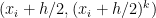
Using the Trapezoid Rule, we approximate as , using the width and the bases and of the trapezoid. Using the Binomial Theorem, this expands as
Once again, this is a little bit overkill for the present purposes, but we’ll need this formula later in this series of posts. Truncating somewhat earlier, we find that the Trapezoid Rule for this subinterval gives
Subtracting from the actual integral, the error in this approximation will be equal to
In other words, like the Midpoint Rule, both of the first two terms and cancel perfectly, leaving us with a local error on the order of .
We also recall, from the previous post in this series that the local error from the Midpoint Rule was . In other words, while both the Midpoint Rule and Trapezoid Rule have local errors on the order of , we expect the error in the Midpoint Rule to be about half of the error from the Trapezoid Rule.
Numerical integration is a standard topic in first-semester calculus. From time to time, I have received questions from students on various aspects of this topic, including:
Why is numerical integration necessary in the first place?
Where do these formulas come from (especially Simpson’s Rule)?
How can I do all of these formulas quickly?
Is there a reason why the Midpoint Rule is better than the Trapezoid Rule?
Is there a reason why both the Midpoint Rule and the Trapezoid Rule converge quadratically?
Is there a reason why Simpson’s Rule converges like the fourth power of the number of subintervals?
In this series, I hope to answer these questions. While these are standard questions in a introductory college course in numerical analysis, and full and rigorous proofs can be found on Wikipedia and Mathworld, I will approach these questions from the point of view of a bright student who is currently enrolled in calculus and hasn’t yet taken real analysis or numerical analysis.
In the previous post, we showed that the midpoint approximation of has error
In this post, we consider the global error when integrating on the interval instead of a subinterval . The logic for determining the global error is much the same as what we used earlier for the left-endpoint rule.
The total error when approximating will be the sum of the errors for the integrals over , , through . Therefore, the total error will be
.
So that this formula doesn’t appear completely mystical, this actually matches the numerical observations that we made earlier. The figure below shows the left-endpoint approximations to for different numbers of subintervals. If we take and , then the error should be approximately equal to
,
which, as expected, is close to the actual error of .
Let , so that the error becomes
,
where is the average of the . Clearly, this average is somewhere between the smallest and the largest of the . Since is a continuous function, that means that there must be some value of between and — and therefore between and — so that by the Intermediate Value Theorem. We conclude that the error can be written as
,
Finally, since is the length of one subinterval, we see that is the total length of the interval . Therefore,
,
where the constant is determined by , , and . In other words, for the special case , we have established that the error from the Midpoint Rule is approximately quadratic in — without resorting to the generalized mean-value theorem and confirming the numerical observations we made earlier.
Numerical integration is a standard topic in first-semester calculus. From time to time, I have received questions from students on various aspects of this topic, including:
Why is numerical integration necessary in the first place?
Where do these formulas come from (especially Simpson’s Rule)?
How can I do all of these formulas quickly?
Is there a reason why the Midpoint Rule is better than the Trapezoid Rule?
Is there a reason why both the Midpoint Rule and the Trapezoid Rule converge quadratically?
Is there a reason why Simpson’s Rule converges like the fourth power of the number of subintervals?
In this series, I hope to answer these questions. While these are standard questions in a introductory college course in numerical analysis, and full and rigorous proofs can be found on Wikipedia and Mathworld, I will approach these questions from the point of view of a bright student who is currently enrolled in calculus and hasn’t yet taken real analysis or numerical analysis.
In this post, we will perform an error analysis for the Midpoint Rule
where is the number of subintervals and is the width of each subinterval, so that . Also, is the midpoint of the th subinterval.
As noted above, a true exploration of error analysis requires the generalized mean-value theorem, which perhaps a bit much for a talented high school student learning about this technique for the first time. That said, the ideas behind the proof are accessible to high school students, using only ideas from the secondary curriculum (especially the Binomial Theorem), if we restrict our attention to the special case , where is a positive integer.
For this special case, the true area under the curve on the subinterval will be
In the above, the shorthand can be formally defined, but here we’ll just take it to mean “terms that have a factor of or higher that we’re too lazy to write out.” Since is supposed to be a small number, these terms will small in magnitude and thus can be safely ignored.
I wrote the above formula to include terms up to and including because I’ll need this later in this series of posts. For now, looking only at the Midpoint Rule, it will suffice to write this integral as
.
Using the midpoint of the subinterval, the left-endpoint approximation of is . Using the Binomial Theorem, this expands as
Once again, this is a little bit overkill for the present purposes, but we’ll need this formula later in this series of posts. Truncating somewhat earlier, we find that the Midpoint Rule for this subinterval gives
Subtracting from the actual integral, the error in this approximation will be equal to
In other words, unlike the left-endpoint and right-endpoint approximations, both of the first two terms and cancel perfectly, leaving us with a local error on the order of .
The logic for determining the global error is much the same as what we used earlier for the left-endpoint rule.
The total error when approximating will be the sum of the errors for the integrals over , , through . Therefore, the total error will be
.
So that this formula doesn’t appear completely mystical, this actually matches the numerical observations that we made earlier. The figure below shows the left-endpoint approximations to for different numbers of subintervals. If we take and , then the error should be approximately equal to
,
which, as expected, is close to the actual error of .
Let , so that the error becomes
,
where is the average of the . Clearly, this average is somewhere between the smallest and the largest of the . Since is a continuous function, that means that there must be some value of between and — and therefore between and — so that by the Intermediate Value Theorem. We conclude that the error can be written as
,
Finally, since is the length of one subinterval, we see that is the total length of the interval . Therefore,
,
where the constant is determined by , , and . In other words, for the special case , we have established that the error from the Midpoint Rule is approximately quadratic in — without resorting to the generalized mean-value theorem and confirming the numerical observations we made earlier.
Numerical integration is a standard topic in first-semester calculus. From time to time, I have received questions from students on various aspects of this topic, including:
Why is numerical integration necessary in the first place?
Where do these formulas come from (especially Simpson’s Rule)?
How can I do all of these formulas quickly?
Is there a reason why the Midpoint Rule is better than the Trapezoid Rule?
Is there a reason why both the Midpoint Rule and the Trapezoid Rule converge quadratically?
Is there a reason why Simpson’s Rule converges like the fourth power of the number of subintervals?
In this series, I hope to answer these questions. While these are standard questions in a introductory college course in numerical analysis, and full and rigorous proofs can be found on Wikipedia and Mathworld, I will approach these questions from the point of view of a bright student who is currently enrolled in calculus and hasn’t yet taken real analysis or numerical analysis.
In the previous post in this series, we found that the local error of the right endpoint approximation to was equal to
.
We now consider the global error when integrating over the interval and not just a particular subinterval.
The total error when approximating will be the sum of the errors for the integrals over , , through . Therefore, the total error will be
.
So that this formula doesn’t appear completely mystical, this actually matches the numerical observations that we made earlier. The figure below shows the left-endpoint approximations to for different numbers of subintervals. If we take and , then the error should be approximately equal to
,
which, as expected, is close to the actual error of .
We now perform a more detailed analysis of the global error, which is almost a perfect copy-and-paste from the previous analysis. Let , so that the error becomes
,
where is the average of the . Clearly, this average is somewhere between the smallest and the largest of the . Since is a continuous function, that means that there must be some value of between and — and therefore between and — so that by the Intermediate Value Theorem. We conclude that the error can be written as
,
Finally, since is the length of one subinterval, we see that is the total length of the interval . Therefore,
,
where the constant is determined by , , and . In other words, for the special case , we have established that the error from the left-endpoint rule is approximately linear in — without resorting to the generalized mean-value theorem.


 cannot be expressed using finitely many elementary functions. Therefore, we must resort to numerical methods instead.


 subintervals provides a better approximation to
  than the normalcdf function.
 . We obtained these approximations using only techniques within the reach of a talented high school student who has mastered Precalculus — especially the Binomial Theorem — and elementary techniques of integration.
 (and, by an easy extension, any polynomial), the formulas that we do obtain easily foreshadow the actual formulas found on Wikipedia or Mathworld or calculus textbooks, thus (hopefully) taking some of the mystery out of these formulas.
 ,
, is some number between
  and
and  . By comparison,
 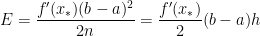 .
. .
. ,
, .
. .
. ,
, .
. ,
, .
. .
. has an error of
 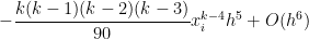 .
.![[a,b]](https://s0.wp.com/latex.php?latex=%5Ba%2Cb%5D&bg=ffffff&fg=000000&s=0&c=20201002) instead of a subinterval
instead of a subinterval ![[x_i,x_i+2h]](https://s0.wp.com/latex.php?latex=%5Bx_i%2Cx_i%2B2h%5D&bg=ffffff&fg=000000&s=0&c=20201002) .
The total error when approximating
.
The total error when approximating  will be the sum of the errors for the integrals over
 ![[x_0,x_2]](https://s0.wp.com/latex.php?latex=%5Bx_0%2Cx_2%5D&bg=ffffff&fg=000000&s=0&c=20201002) ,
, ![[x_2,x_4]](https://s0.wp.com/latex.php?latex=%5Bx_2%2Cx_4%5D&bg=ffffff&fg=000000&s=0&c=20201002) , through
, through ![[x_{n-2},x_n]](https://s0.wp.com/latex.php?latex=%5Bx_%7Bn-2%7D%2Cx_n%5D&bg=ffffff&fg=000000&s=0&c=20201002) . Therefore, the total error will be
. Therefore, the total error will be
 for different numbers of subintervals. If we take
  and
and  , then the error should be approximately equal to
 ,
, .
.
 , so that the error becomes
 ,
, is the average of the
  . (We notice that there are only
  terms in this sum since we’re adding only the even terms.) Clearly, this average is somewhere between the smallest and the largest of the
  is a continuous function, that means that there must be some value of
  and
and  — and therefore between
  by the Intermediate Value Theorem. We conclude that the error can be written as
 ,
, is the length of one subinterval, we see that
  is the total length of the interval
 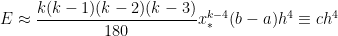 ,
, is determined by
  . In other words, for the special case
 ![\int_a^b f(x) \, dx \approx \frac{h}{3} \left[f(x_0) + 4(x_1) + 2f(x_2) + \dots + 2f(x_{n-2}) + 4f(x_{n-1}) +f(x_n) \right] \equiv T_n](https://s0.wp.com/latex.php?latex=%5Cint_a%5Eb+f%28x%29+%5C%2C+dx+%5Capprox+%5Cfrac%7Bh%7D%7B3%7D+%5Cleft%5Bf%28x_0%29+%2B+4%28x_1%29+%2B+2f%28x_2%29+%2B+%5Cdots+%2B+2f%28x_%7Bn-2%7D%29+%2B+4f%28x_%7Bn-1%7D%29+%2Bf%28x_n%29+%5Cright%5D+%5Cequiv+T_n&bg=ffffff&fg=000000&s=0&c=20201002)
 is the number of subintervals (which has to be even) and
  is the width of each subinterval, so that
  .
.
 is a positive integer.
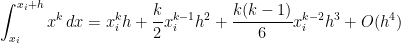
![[x_i, x_i +h]](https://s0.wp.com/latex.php?latex=%5Bx_i%2C+x_i+%2Bh%5D&bg=ffffff&fg=000000&s=0&c=20201002) will be
will be![\displaystyle \int_{x_i}^{x_i+h} x^k \, dx = \frac{1}{k+1} \left[ (x_i+h)^{k+1} - x_i^{k+1} \right]](https://s0.wp.com/latex.php?latex=%5Cdisplaystyle+%5Cint_%7Bx_i%7D%5E%7Bx_i%2Bh%7D+x%5Ek+%5C%2C+dx+%3D+%5Cfrac%7B1%7D%7Bk%2B1%7D+%5Cleft%5B+%28x_i%2Bh%29%5E%7Bk%2B1%7D+-+x_i%5E%7Bk%2B1%7D+%5Cright%5D&bg=ffffff&fg=000000&s=0&c=20201002)
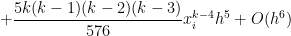
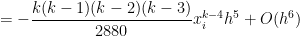
![= \displaystyle \frac{1}{k+1} \left[x_i^{k+1} + {k+1 \choose 1} x_i^k h + {k+1 \choose 2} x_i^{k-1} h^2 + {k+1 \choose 3} x_i^{k-2} h^3 + {k+1 \choose 4} x_i^{k-3} h^4+ {k+1 \choose 5} x_i^{k-4} h^5+ O(h^6) - x_i^{k+1} \right]](https://s0.wp.com/latex.php?latex=%3D+%5Cdisplaystyle+%5Cfrac%7B1%7D%7Bk%2B1%7D+%5Cleft%5Bx_i%5E%7Bk%2B1%7D+%2B+%7Bk%2B1+%5Cchoose+1%7D+x_i%5Ek+h+%2B+%7Bk%2B1+%5Cchoose+2%7D+x_i%5E%7Bk-1%7D+h%5E2+%2B+%7Bk%2B1+%5Cchoose+3%7D+x_i%5E%7Bk-2%7D+h%5E3+%2B+%7Bk%2B1+%5Cchoose+4%7D+x_i%5E%7Bk-3%7D+h%5E4%2B+%7Bk%2B1+%5Cchoose+5%7D+x_i%5E%7Bk-4%7D+h%5E5%2B+O%28h%5E6%29+-+x_i%5E%7Bk%2B1%7D+%5Cright%5D&bg=ffffff&fg=000000&s=0&c=20201002)

![+ \displaystyle \frac{(k+1)k(k-1)(k-2)(k-3)}{120} x_i^{k-4} h^5 \bigg] + O(h^6)](https://s0.wp.com/latex.php?latex=%2B+%5Cdisplaystyle+%5Cfrac%7B%28k%2B1%29k%28k-1%29%28k-2%29%28k-3%29%7D%7B120%7D+x_i%5E%7Bk-4%7D+h%5E5+%5Cbigg%5D+%2B+O%28h%5E6%29+&bg=ffffff&fg=000000&s=0&c=20201002)

 can be formally defined, but here we’ll just take it to mean “terms that have a factor of
  or higher that we’re too lazy to write out.” Since
  relating the approximations from Simpson’s Rule, the Midpoint Rule, and the Trapezoid Rule. We now exploit this relationship to approximate
  . Earlier in this series, we found the Midpoint Rule approximation on this subinterval to be


 .
. subintervals, the Simpson’s Rule approximation of
  ,
,  , and
, and  — will be
 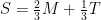 . Since
 ,
, ,
, ,
,
 .
. perfectly match the first four terms of the exact value of the integral! Subtracting from the actual integral, the error in this approximation will be equal to

 , where
  and
and  , where only
 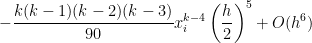 ,
, is the width of all of the
  , a vast improvement over both the Midpoint Rule and the Trapezoid Rule. This illustrates a general principle of numerical analysis: given two algorithms that are
  , an improved algorithm can typically be made by taking some linear combination of the two algorithms. Usually, the improvement will be to
  ; however, in this example, we magically obtained an improvement to
![[x_i,x_i+h]](https://s0.wp.com/latex.php?latex=%5Bx_i%2Cx_i%2Bh%5D&bg=ffffff&fg=000000&s=0&c=20201002) . The logic is almost a perfect copy-and-paste from the analysis used for the Midpoint Rule.
The total error when approximating
. The logic is almost a perfect copy-and-paste from the analysis used for the Midpoint Rule.
The total error when approximating ![[x_0,x_1]](https://s0.wp.com/latex.php?latex=%5Bx_0%2Cx_1%5D&bg=ffffff&fg=000000&s=0&c=20201002) ,
, ![[x_1,x_2]](https://s0.wp.com/latex.php?latex=%5Bx_1%2Cx_2%5D&bg=ffffff&fg=000000&s=0&c=20201002) , through
, through ![[x_{n-1},x_n]](https://s0.wp.com/latex.php?latex=%5Bx_%7Bn-1%7D%2Cx_n%5D&bg=ffffff&fg=000000&s=0&c=20201002) . Therefore, the total error will be
. Therefore, the total error will be
 .
. ,
, .
.
 , so that the error becomes
 ,
, is the average of the
  is a continuous function, that means that there must be some value of
  — and therefore between
  by the Intermediate Value Theorem. We conclude that the error can be written as
 ,
, ,
,![\int_a^b f(x) \, dx \approx \frac{h}{2} \left[f(x_0) + 2f(x_1) + 2f(x_2) + \dots + 2f(x_{n-1}) +f(x_n) \right] \equiv T_n](https://s0.wp.com/latex.php?latex=%5Cint_a%5Eb+f%28x%29+%5C%2C+dx+%5Capprox+%5Cfrac%7Bh%7D%7B2%7D+%5Cleft%5Bf%28x_0%29+%2B+2f%28x_1%29+%2B+2f%28x_2%29+%2B+%5Cdots+%2B+2f%28x_%7Bn-1%7D%29+%2Bf%28x_n%29+%5Cright%5D+%5Cequiv+T_n&bg=ffffff&fg=000000&s=0&c=20201002)
 because I’ll need this later in this series of posts. For now, looking only at the Trapezoid Rule, it will suffice to write this integral as
 .
.![\displaystyle \frac{h}{2} \left[x_i^k + (x_i + h)^k \right]](https://s0.wp.com/latex.php?latex=%5Cdisplaystyle+%5Cfrac%7Bh%7D%7B2%7D+%5Cleft%5Bx_i%5Ek+%2B+%28x_i+%2B+h%29%5Ek+%5Cright%5D&bg=ffffff&fg=000000&s=0&c=20201002) , using the width
, using the width  and
and  of the trapezoid. Using the Binomial Theorem, this expands as


 and
and  cancel perfectly, leaving us with a local error on the order of
  .
We also recall, from the previous post in this series that the local error from the Midpoint Rule was
.
We also recall, from the previous post in this series that the local error from the Midpoint Rule was 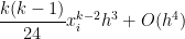 . In other words, while both the Midpoint Rule and Trapezoid Rule have local errors on the order of
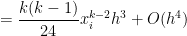
 .
. ,
, .
.
 ,
, ,
, ,
,![\int_a^b f(x) \, dx \approx h \left[f(c_1) + f(c_2) + \dots + f(c_n) \right] \equiv M_n](https://s0.wp.com/latex.php?latex=%5Cint_a%5Eb+f%28x%29+%5C%2C+dx+%5Capprox+h+%5Cleft%5Bf%28c_1%29+%2B+f%28c_2%29+%2B+%5Cdots+%2B+f%28c_n%29+%5Cright%5D+%5Cequiv+M_n&bg=ffffff&fg=000000&s=0&c=20201002)
 is the midpoint of the
  th subinterval.

 . Using the Binomial Theorem, this expands as


 .
. will be the sum of the errors for the integrals over
  .
. ,
, .
.
 , so that the error becomes
 ,
, is the average of the
  is a continuous function, that means that there must be some value of
  and
and  — and therefore between
  by the Intermediate Value Theorem. We conclude that the error can be written as
 ,
, ,
,