Lagrange Points and Polynomial Equations: Part 1

I recently read a terrific article in the American Mathematical Monthly about Lagrange points, which are (from Wikipedia) “points of equilibrium for small-mass objects under the gravitational influence of two massive orbiting bodies.” There are five such points in the Sun-Earth system, called $L_1$ , $L_2$ , $L_3$ , $L_4$ , and $L_5$ .

To describe these Lagrange points, I can do no better than the estimable Isaac Asimov. I quote from his essay “Colonizing the Heavens” from his book The Beginning and the End, which was published in 1977. I read the book over and over again as a boy in the mid-1980s. (Asimov’s essay originally concerned the Earth-Moon system; in the quote below, I changed the words to apply to the Sun-Earth system.)

Imagine the Sun at zenith, exactly overhead. Trace a line due eastward from the Sun down to the horizon. Two-thirds of the way along that line, one-third of the way up from the horizon, is one of those places. Trace another line westward away from the Sun down to the horizon. Two-thirds of the way along that line, one-third of the way up from the horizon, is another of those places.

Put an object in either place and it will form an equilateral triangle with the Sun and Earth…

What is so special about those places? Back in 1772, the astronomer Joseph Louis Lagrange showed that in those places any object remained stationary with respect to the Sun. As the Earth moved about the Sun, any object in either of those places would also move about the Sun in such a way as to keep perfect step with the Earth. The competing gravities of the Sun and Earth would keep it where it was. If anything happened to push it out of place it would promptly move back, wobbling back and forth a bit (“librating”) as it did so. The two places are called “Lagrangian points” or “libration points.”

Lagrange discovered five such places altogether, but three of them are of no importance since they don’t represent stable conditions. An object in those three places, once pushed out of place, would continue to drift outward and would never return.

The last paragraph of the above quote represents a rare failure of imagination by Asimov, who wrote prolifically about the future of spaceflight. Points $L_4$ and $L_5$ are indeed stable equilibria, and untold science fiction stories have placed spacecraft or colonies at these locations. (The rest of Asimov’s essay speculates about using these points in the Earth-Moon system for space colonization.) However, while the points $L_1$ and $L_2$ are unstable equilibria, they do have practical applications for spacecraft that can perform minor course corrections to stay in position. (The point $L_3$ is especially unstable to outside gravitational influences and thus seems unsuitable for spacecraft.) Again from Wikipedia,

Sun–Earth L₁ is suited for making observations of the Sun–Earth system. Objects here are never shadowed by Earth or the Moon and, if observing Earth, always view the sunlit hemisphere… Solar and heliospheric missions currently located around L₁ include the Solar and Heliospheric Observatory, Wind, Aditya-L1 Mission and the Advanced Composition Explorer. Planned missions include the Interstellar Mapping and Acceleration Probe(IMAP) and the NEO Surveyor.

Sun–Earth L₂ is a good spot for space-based observatories. Because an object around L₂ will maintain the same relative position with respect to the Sun and Earth, shielding and calibration are much simpler… The James Webb Space Telescope was positioned in a halo orbit about L₂ on January 24, 2022.

Earth–Moon L₁ allows comparatively easy access to Lunar and Earth orbits with minimal change in velocity and this has as an advantage to position a habitable space station intended to help transport cargo and personnel to the Moon and back. The SMART-1 Mission passed through the L₁ Lagrangian Point on 11 November 2004 and passed into the area dominated by the Moon’s gravitational influence.

Earth–Moon L₂ has been used for a communications satellite covering the Moon’s far side, for example, Queqiao, launched in 2018, and would be “an ideal location” for a propellant depot as part of the proposed depot-based space transportation architecture.

While the locations $L_4$ and $L_5$ are easy to describe, the precise locations of $L_1$ and $L_2$ are found by numerically solving a fifth-order polynomial equation. This was news to me when I read that article from the American Mathematical Monthly. While I had read years ago that finding the positions of the other three Lagrange points wasn’t simple, I did not realize that it was no more complicated that numerically finding the roots of a polynomial.

The above article from the American Mathematical Monthly concludes…

[t]he mathematical tools that Lagrange uses to arrive at a solution to this three-body problem lie entirely within the scope of modern courses in algebra, trigonometry, and first-semester calculus. But surely no ordinary person could have pursued the many extraordinarily complicated threads in his work to their ends, let alone woven them together into a magnificent solution to the problem as he has done. Lagrange noted in the introduction to his essay, “This research is really no more than for pure curiosity …” If only he could have watched on Christmas Day as the James Webb Space Telescope began its journey to the Lagrange point $L_2$ !

In this short series, we discuss the polynomial equations for finding $L_1$ and $L_2$ .

Definition of e

Source: https://xkcd.com/2768

Confirming Einstein’s Theory of General Relativity With Calculus, Part 3: Method of Successive Approximations

In this series, I’m discussing how ideas from calculus and precalculus (with a touch of differential equations) can predict the precession in Mercury’s orbit and thus confirm Einstein’s theory of general relativity. The origins of this series came from a class project that I assigned to my Differential Equations students maybe 20 years ago.

One technique that will be necessary for this confirmation is the method of successive approximations. This will be needed in the context of a differential equation; however, we can illustrate the concept by finding the roots of a polynomial. Consider the quadratic equation

$x^2 - x - 1 = 0$ .

(Naturally, we can solve for $x$ using the quadratic formula; more on that later.) To apply the method of successive approximation, we will rewrite this so that $x$ appears on the left side and some function of $x$ appears on the right side. I will choose

$x^2 = x + 1$ , or

$x = 1 + \displaystyle \frac{1}{x}$ .

Here’s the idea of the method of successive approximations to obtain a recursively defined sequence that (hopefully) convergence to a solution of this equation:

Start with an initial guess $x_0$ .
Plug $x_0$ into the right-hand side to get a new guess, $x_1$ .
Plug $x_1$ into the right-hand side to get a new guess, $x_2$ .
And repeat.

For example, suppose that we choose $x_0 = 1$ . Then

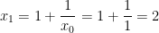
$x_1 = 1 + \displaystyle \frac{1}{x_0} = 1 + \displaystyle \frac{1}{1} = 2$

$x_2 = 1 + \displaystyle \frac{1}{x_1} = 1 + \displaystyle \frac{1}{2} = \displaystyle \frac{3}{2} = 1.5$

$x_3 = 1 + \displaystyle \frac{1}{x_2} = 1 + \displaystyle \frac{1}{3/2} = \displaystyle \frac{5}{3} \approx 1.667$

$x_4 = 1 + \displaystyle \frac{1}{x_3} = 1 + \displaystyle \frac{1}{5/3} = \displaystyle \frac{8}{5} = 1.6$

$x_5 = 1 + \displaystyle \frac{1}{x_4} = 1 + \displaystyle \frac{1}{8/5} = \displaystyle \frac{13}{8} = 1.625$

$x_6 = 1 + \displaystyle \frac{1}{x_5} = 1 + \displaystyle \frac{1}{13/8} = \displaystyle \frac{21}{13} \approx 1.615$

$x_7 = 1 + \displaystyle \frac{1}{x_6} = 1 + \displaystyle \frac{1}{21/13} = \displaystyle \frac{34}{21} \approx 1.619$

This sequence can be computed by entering $1$ into a calculator, then entering $1 + 1 \div \hbox{Ans}$ , and then repeatedly hitting the $=$ button.

We see that the sequence appears to be converging to something, and that something is a root of the equation $x^2 - x - 1 = 0$ , which we now find via the quadratic formula:

$x = \displaystyle \frac{1 \pm \sqrt{1 - 4 \cdot 1 \cdot (-1)}}{2} = \frac{1 \pm \sqrt{5}}{2}$ .

So it looks like the above sequence is converging to the positive root $(1 + \sqrt{5})/2 \approx 1.618$ .

(Parenthetically, you might notice that the Fibonacci sequence appears in the numerators and denominators of this sequence. As you might guess, that’s not a coincidence.)

Like most numerical techniques, this method doesn’t always work like we think it would. Another solution is the negative root $(1 - \sqrt{5})/2 \approx -0.618$ . Unfortunately, if we start with a guess near this root, like $x_0 = -0.62$ , the sequence unexpectedly diverges from $-0.618\dots$ but eventually converges to the positive root $1.618\dots$ :

$x_1 = 1 + \displaystyle \frac{1}{x_0} = 1 + \displaystyle \frac{1}{-0.62} = -0.6129\dots$

$x_2 = 1 + \displaystyle \frac{1}{x_1} = 1 + \displaystyle \frac{1}{-0.6129\dots} = -0.6315\dots$

$x_3 = 1 + \displaystyle \frac{1}{x_2} = 1 + \displaystyle \frac{1}{-0.6315\dots} = -0.5833\dots$

$x_4 = 1 + \displaystyle \frac{1}{x_3} = 1 + \displaystyle \frac{1}{-0.5833\dots} = -0.7142\dots$

$x_5 = 1 + \displaystyle \frac{1}{x_4} = 1 + \displaystyle \frac{1}{-0.5833\dots} = -0.4$

$x_6 = 1 + \displaystyle \frac{1}{x_5} = 1 + \displaystyle \frac{1}{-0.4\dots} = -1.5$

$x_7 = 1 + \displaystyle \frac{1}{x_6} = 1 + \displaystyle \frac{1}{-1.5\dots} = 0.3333\dots$

$x_8 = 1 + \displaystyle \frac{1}{x_7} = 1 + \displaystyle \frac{1}{0.3333\dots} = 4$

$x_9 = 1 + \displaystyle \frac{1}{x_8} = 1 + \displaystyle \frac{1}{4} = 1.25$

$x_{10} = 1 + \displaystyle \frac{1}{x_9} = 1 + \displaystyle \frac{1}{1.25} = 1.8$

$x_{11} = 1 + \displaystyle \frac{1}{x_{10}} = 1 + \displaystyle \frac{1}{1.8} = 1.555\dots$

$x_{12} = 1 + \displaystyle \frac{1}{x_{11}} = 1 + \displaystyle \frac{1}{1.555\dots} = 1.6428\dots$

$x_{13} = 1 + \displaystyle \frac{1}{x_{12}} = 1 + \displaystyle \frac{1}{1.6428\dots} = 1.6086\dots$

$x_{14} = 1 + \displaystyle \frac{1}{x_{13}} = 1 + \displaystyle \frac{1}{1.6086\dots} = 1.6216\dots$

$x_{15} = 1 + \displaystyle \frac{1}{x_{14}} = 1 + \displaystyle \frac{1}{1.6216\dots} = 1.6166\dots$

$x_{16} = 1 + \displaystyle \frac{1}{x_{15}} = 1 + \displaystyle \frac{1}{1.6216\dots} = 1.6185\dots$

I should note that the method of successive approximations generally converges at a slower pace than Newton’s method. However, this method will be good enough when we use it to predict the precession in Mercury’s orbit.

Parabolas from String Art: Index

I’m doing something that I should have done a long time ago: collecting a series of posts into one single post. The links below show my series on numerical integration.

Part 1: Introduction

Part 2: Identifying the highest points of the strings

Part 3: These nine points lie on a parabola: Method #1

Part 4: These nine points lie on a parabola: Method #2

Part 5: These nine points lie on a parabola: Method #3

Part 6: Proof that all of the highest points lie on a parabola without calculus, Part 1

Part 7: Proof that all of the highest points lie on a parabola without calculus, Part 2

Part 8: Proof that all of the highest points lie on a parabola with calculus

Part 9: Proof that the strings are indeed tangent to the parabola, with calculus

Part 10: Conclusion

Square roots and Logarithms Without a Calculator: Index

I’m doing something that I should have done a long time ago: collect past series of posts into a single, easy-to-reference post. The following posts formed my series on computing square roots and logarithms without a calculator (with the latest post added).

Part 1: Method #1: Trial and error.

Part 2: Method #2: An algorithm comparable to long division.

Part 3: Method #3: Introduction to logarithmic tables.

Part 4: Finding antilogarithms with a table.

Part 5: Pedagogical and historical thoughts on log tables.

Part 6: Computation of square roots using a log table.

Part 7: Method #4: Slide rules

Part 8: Method #5: By hand, using a couple of known logarithms base 10, the change of base formula, and the Taylor approximation $\ln(1+x) \approx x$ .

Part 9: An in-class activity for getting students comfortable with logarithms when seen for the first time.

Part 10: Method #6: Mentally… anecdotes from Nobel Prize-winning physicist Richard P. Feynman and me.

Part 11: Method #7: Newton’s Method.

Part 12: Method #8: The formula $\sqrt{b} \approx \displaystyle \frac{a+b}{2\sqrt{a}}$

More fun with logarithmic scales

Source: https://xkcd.com/2711/

Parabolas from String Art (Part 10)

Recently, I announced that my paper Parabolic Properties from Pieces of String had been published in the magazine Math Horizons. The article had multiple aims; in chronological order of when I first started thinking about them:

Prove that string art from two line segments traces a parabola.
Prove that a quadratic polynomial satisfies the focus-directrix property of a parabola, which is the reverse of the usual logic when students learn conic sections.
Prove the reflective property of parabolas.
Accomplish all of the above without using calculus.

While I’m generally pleased with the final form of the article, the necessity of publication constraints somewhat abbreviated the original goal of this project: determining a pedagogically sound way of convincing a bright Algebra I student that string art unexpectedly produces a parabola. In this series of posts, I’d wanted to expand on the article with some pedagogical thoughts about connecting string art to parabolas for algebra students. After all, most mathematical studies of string art curves — formally known as “envelopes” — rely on differential equations or at least limits and calculus.

However, string art is simple enough for a young child to construct, and so this study was inspired by the quest of explaining this phenomenon using only simple mathematical tools.

The article linked above has further thoughts on this problem, including a calculus-free way of deriving the reflective property of parabolas. However, I think the article pretty much has all of my thoughts on this matter, and so I don’t think I need to elaborate upon them here.

This series of posts is dedicated to an inspired and inspiring Algebra I student who wanted to understand string art curves using tools that she could understand… even though she progressed much further into the mathematics curriculum by the time my article was published and this series of posts appeared on my blog.

Parabolas from String Art (Part 9)

Prove that string art from two line segments traces a parabola.
Prove that a quadratic polynomial satisfies the focus-directrix property of a parabola, which is the reverse of the usual logic when students learn conic sections.
Prove the reflective property of parabolas.
Accomplish all of the above without using calculus.

While I’m generally pleased with the final form of the article, the necessity of publication constraints somewhat abbreviated the original goal of this project: determining a pedagogically sound way of convincing a bright Algebra I student that string art unexpectedly produces a parabola. While all the necessary mathematics is in the article, I think the article is somewhat lacking on how to sell the idea to students. So, in this series of posts, I’d like to expand on the article with some pedagogical thoughts about connecting string art to parabolas.

We have shown in the last couple of posts that if the three points that generate the Our explorations of string art led us to consider an arbitrary string $\overline{PQ}$ depicted below. For brevity, this string will be called “string $s$ ,” matching the (possibly non-integer) $x$ -coordinate of its left endpoint $P$ . Since $P$ is $s$ units to the right of $A$ , the right endpoint $Q$ must correspondingly be $s$ units to the right of $B$ . Therefore, the $x$ -coordinate of $Q$ is $s + 8$ .

Previously, we established that the equation for string $s$ is

$y = -\displaystyle \frac{s^2}{4} + \frac{xs}{4} - x + 8$ .

We also obtained a bonus result that we obtained using only algebra: string $s$ is tangent to the parabola $y = \displaystyle \frac{x^2}{16} - x + 8$ , which is traced by the strings, when $x=2s$ . Of course, tangent lines are usually obtained using calculus, and so calculus should be able to confirm this result. The derivative of this function is

$y' = \displaystyle \frac{x}{8} - 1$ ,

so that the slope of the tangent line when $x=2s$ is $m = \displaystyle \frac{s}{4} - 1 = \frac{s-4}{4}$ . We observe that this matches the slope of line segment $\overline{PQ}$ in the above picture:

slope $= \displaystyle \frac{s - (s-8)}{(s+8) - 8} = \frac{2s-8}{8} = \frac{s-4}{4}$ .

Therefore, to show that $\overline{PQ}$ is the tangent line, it suffices to show that either $P$ or $Q$ is on the tangent line.

At $x = 2s$ , the $y-$ coordinate of where the tangent line intersects the curve is

$y = \displaystyle \frac{(2s)^2}{16} - 2s + 8 = \frac{s^2}{4} - 2s + 8$ .

Using the point-slope formula for a line, the equation of the tangent line is thus

$y-y_1 = m(x-x_1)$

$y-\displaystyle \left( \frac{s^2}{4} - 2s + 8 \right) = \frac{s-4}{4} (x-2s)$

$y = \displaystyle \frac{s-4}{4} (x-2s) + \frac{s^2}{4} - 2s + 8$ .

We now check to see if $P(s,8-s)$ is on the tangent line. Substituting $x =s$ , we find

$y = \displaystyle \frac{s-4}{4} (s-2s) + \frac{s^2}{4} - 2s + 8$

$= \displaystyle \frac{s-4}{4} (-s) + \frac{s^2}{4} - 2s + 8$

$= \displaystyle \frac{(s-4)(-s) + s^2}{4} - 2s + 8$

$= \displaystyle \frac{-s^2+4s + s^2}{4} - 2s + 8$

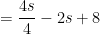
$= \displaystyle \frac{4s}{4} - 2s + 8$

$= s - 2s + 8$

$= -s + 8$

Therefore, the point $(s,8-s)$ is on the tangent line, thus confirming that $P$ is on the tangent line and that $\overline{PQ}$ is the tangent line.

Parabolas from String Art (Part 8)

Prove that string art from two line segments traces a parabola.
Prove that a quadratic polynomial satisfies the focus-directrix property of a parabola, which is the reverse of the usual logic when students learn conic sections.
Prove the reflective property of parabolas.
Accomplish all of the above without using calculus.

While I’m generally pleased with the final form of the article, the necessity of publication constraints somewhat abbreviated the original goal of this project: determining a pedagogically sound way of convincing a bright Algebra I student that string art unexpectedly produces a parabola. While all the necessary mathematics is in the article, I think the article is somewhat lacking on how to sell the idea to students. So, in this series of posts, I’d like to expand on the article with some pedagogical thoughts about connecting string art to parabolas.

Previously, we established that the equation for string $s$ is

$y = -\displaystyle \frac{s^2}{4} + \frac{xs}{4} - x + 8$ .

Finding the curve traced by the strings is a two-step process:

For a fixed value of $x$ , find the value of $s$ that maximizes $y$ .
Find this optimal value of $y$ .

Previously, we showed using only algebra that the optimal value of $s$ is $s = \displaystyle \frac{x}{2}$ , corresponding to an optimal value of $y$ of $y = \displaystyle \frac{x^2}{16} - x + 8$ .

For a student who knows calculus, the optimal value of $s$ can be found by instead solving the equation $\displaystyle \frac{dy}{ds} = 0$ (or, more accurately, $\displaystyle \frac{\partial y}{\partial s} = 0$ ):

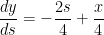
$\displaystyle \frac{dy}{ds} = -\frac{2s}{4} + \frac{x}{4}$

$0 = \displaystyle \frac{-2s+x}{4}$

$0 = -2s + x$

$2s = x$

$s = \displaystyle \frac{x}{2}$ ,

matching the result that we found by using only algebra.

Parabolas from String Art (Part 7)

Prove that string art from two line segments traces a parabola.
Prove that a quadratic polynomial satisfies the focus-directrix property of a parabola, which is the reverse of the usual logic when students learn conic sections.
Prove the reflective property of parabolas.
Accomplish all of the above without using calculus.

While I’m generally pleased with the final form of the article, the necessity of publication constraints somewhat abbreviated the original goal of this project: determining a pedagogically sound way of convincing a bright Algebra I student that string art unexpectedly produces a parabola. While all the necessary mathematics is in the article, I think the article is somewhat lacking on how to sell the idea to students. So, in this series of posts, I’d like to expand on the article with some pedagogical thoughts about connecting string art to parabolas.

Our explorations of string art led us to consider an arbitrary string $\overline{PQ}$ depicted below. For brevity, this string will be called “string $s$ ,” matching the (possibly non-integer) $x$ -coordinate of its left endpoint $P$ . Since $P$ is $s$ units to the right of $A$ , the right endpoint $Q$ must correspondingly be $s$ units to the right of $B$ . Therefore, the $x$ -coordinate of $Q$ is $s + 8$ .

In the previous post, we established that the equation for string $s$ is

$y = -\displaystyle \frac{s^2}{4} + \frac{xs}{4} - x + 8$

This has the appearance of a quadratic equation, but it’s actually a linear equation in $x$ for a fixed value of $s$ . For example, if s = 5, we find that the equation of string 5 is

$y = -\displaystyle \frac{25}{4} + \frac{5x}{4} - x +8 = 0.25x+1.75$ ,

matching the equation of the blue string we found in a previous post in this series.

To prove that the strings trace a parabola, we now determine which string $s$ maximizes the value of $y = -\displaystyle \frac{1}{4}s^2 + \frac{x}{4}s - x + 8$ for a given value of $x$ . Algebra students can determine this maximum by recalling that a quadratic function $y = as^2 + bs + c$ is maximized (for negative $a$ ) when $s = \displaystyle -\frac{b}{2a}$ . Therefore, the string with largest $y$ -coordinate for a given value of $x$ is

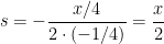
$s = \displaystyle -\frac{x/4}{2 \cdot (-1/4)} = \frac{x}{2}$ .

For example, if $x = 4$ , then string $s = 4 / 2 = 2$ has the largest $y$ -coordinate, matching our previous observations.
To complete the proof that the strings above trace a parabola, we substitute $s = \displaystyle \frac{x}{2}$ into $y = -\displaystyle \frac{s^2}{4} + \frac{xs}{4} - x + 8$ to find the value of this largest $y-$ coordinate:

$y = -\displaystyle \frac{(x/2)^2}{4} + \frac{x(x/2)}{4} - x + 8$

$= -\displaystyle \frac{x^2}{16} + \frac{x^2}{8} - x + 8$

$= \displaystyle \frac{x^2}{16} - x + 8$ ,

matching the result that we found earlier in this series.

There’s also a bonus result. We further note that, for every $x$ , there is only one string $s = \frac{x}{2}$ that intersects the parabola $y = \displaystyle \frac{x^2}{16} - x + 8$ . Since each $x$ is associated with a unique string $s$ and vice versa, we conclude that each string intersects the parabola at exactly one point. In other words, string $s$ is tangent to the parabola $y = \displaystyle \frac{x^2}{16} - x + 8$ when $x=2s$ .

We note that all of the above calculations were entirely elementary, in the sense that calculus was not used and that only techniques from algebra were employed. That said, the word “elementary” in mathematics can be a bit loaded — this means that it is based on simple ideas that are perhaps used in a profound and surprising way. Perhaps my favorite quote along these lines was this understated gem from the book Three Pearls of Number Theory after the conclusion of a very complicated multi-page proof in Chapter 1:

You see how complicated an entirely elementary construction can sometimes be. And yet this is not an extreme case; in the next chapter you will encounter just as elementary a construction which is considerably more complicated.

In the next post, we take a second look at this derivation using techniques from calculus.