- Why is numerical integration necessary in the first place?
- Where do these formulas come from (especially Simpson’s Rule)?
- How can I do all of these formulas quickly?
- Is there a reason why the Midpoint Rule is better than the Trapezoid Rule?
- Is there a reason why both the Midpoint Rule and the Trapezoid Rule converge quadratically?
- Is there a reason why Simpson’s Rule converges like the fourth power of the number of subintervals?

![\int_a^b f(x) \, dx \approx h \left[f(c_1) + f(c_2) + \dots + f(c_n) \right] \equiv M_n](https://s0.wp.com/latex.php?latex=%5Cint_a%5Eb+f%28x%29+%5C%2C+dx+%5Capprox+h+%5Cleft%5Bf%28c_1%29+%2B+f%28c_2%29+%2B+%5Cdots+%2B+f%28c_n%29+%5Cright%5D+%5Cequiv+M_n&bg=ffffff&fg=000000&s=0&c=20201002)
 is the number of subintervals and
  is the width of each subinterval, so that
  . Also,
  is the midpoint of the
  th subinterval.

 , where
  is a positive integer.
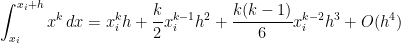
For this special case, the true area under the curve ![[x_i, x_i +h]](https://s0.wp.com/latex.php?latex=%5Bx_i%2C+x_i+%2Bh%5D&bg=ffffff&fg=000000&s=0&c=20201002)
![\displaystyle \int_{x_i}^{x_i+h} x^k \, dx = \frac{1}{k+1} \left[ (x_i+h)^{k+1} - x_i^{k+1} \right]](https://s0.wp.com/latex.php?latex=%5Cdisplaystyle+%5Cint_%7Bx_i%7D%5E%7Bx_i%2Bh%7D+x%5Ek+%5C%2C+dx+%3D+%5Cfrac%7B1%7D%7Bk%2B1%7D+%5Cleft%5B+%28x_i%2Bh%29%5E%7Bk%2B1%7D+-+x_i%5E%7Bk%2B1%7D+%5Cright%5D&bg=ffffff&fg=000000&s=0&c=20201002)
![= \displaystyle \frac{1}{k+1} \left[x_i^{k+1} + {k+1 \choose 1} x_i^k h + {k+1 \choose 2} x_i^{k-1} h^2 + {k+1 \choose 3} x_i^{k-2} h^3 + {k+1 \choose 4} x_i^{k-3} h^4+ {k+1 \choose 5} x_i^{k-4} h^5+ O(h^6) - x_i^{k+1} \right]](https://s0.wp.com/latex.php?latex=%3D+%5Cdisplaystyle+%5Cfrac%7B1%7D%7Bk%2B1%7D+%5Cleft%5Bx_i%5E%7Bk%2B1%7D+%2B+%7Bk%2B1+%5Cchoose+1%7D+x_i%5Ek+h+%2B+%7Bk%2B1+%5Cchoose+2%7D+x_i%5E%7Bk-1%7D+h%5E2+%2B+%7Bk%2B1+%5Cchoose+3%7D+x_i%5E%7Bk-2%7D+h%5E3+%2B+%7Bk%2B1+%5Cchoose+4%7D+x_i%5E%7Bk-3%7D+h%5E4%2B+%7Bk%2B1+%5Cchoose+5%7D+x_i%5E%7Bk-4%7D+h%5E5%2B+O%28h%5E6%29+-+x_i%5E%7Bk%2B1%7D+%5Cright%5D&bg=ffffff&fg=000000&s=0&c=20201002)

![+ \displaystyle \frac{(k+1)k(k-1)(k-2)(k-3)}{120} x_i^{k-4} h^5 \bigg] + O(h^6)](https://s0.wp.com/latex.php?latex=%2B+%5Cdisplaystyle+%5Cfrac%7B%28k%2B1%29k%28k-1%29%28k-2%29%28k-3%29%7D%7B120%7D+x_i%5E%7Bk-4%7D+h%5E5+%5Cbigg%5D+%2B+O%28h%5E6%29+&bg=ffffff&fg=000000&s=0&c=20201002)

 can be formally defined, but here we’ll just take it to mean “terms that have a factor of
  or higher that we’re too lazy to write out.” Since
  is supposed to be a small number, these terms will small in magnitude and thus can be safely ignored.
I wrote the above formula to include terms up to and including
is supposed to be a small number, these terms will small in magnitude and thus can be safely ignored.
I wrote the above formula to include terms up to and including  because I’ll need this later in this series of posts. For now, looking only at the Midpoint Rule, it will suffice to write this integral as
 is
is  . Using the Binomial Theorem, this expands as


 and
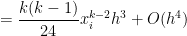
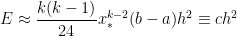
and  cancel perfectly, leaving us with a local error on the order of
  .
.
 will be the sum of the errors for the integrals over
 ![[x_0,x_1]](https://s0.wp.com/latex.php?latex=%5Bx_0%2Cx_1%5D&bg=ffffff&fg=000000&s=0&c=20201002) ,
, ![[x_1,x_2]](https://s0.wp.com/latex.php?latex=%5Bx_1%2Cx_2%5D&bg=ffffff&fg=000000&s=0&c=20201002) , through
, through ![[x_{n-1},x_n]](https://s0.wp.com/latex.php?latex=%5Bx_%7Bn-1%7D%2Cx_n%5D&bg=ffffff&fg=000000&s=0&c=20201002) . Therefore, the total error will be
. Therefore, the total error will be

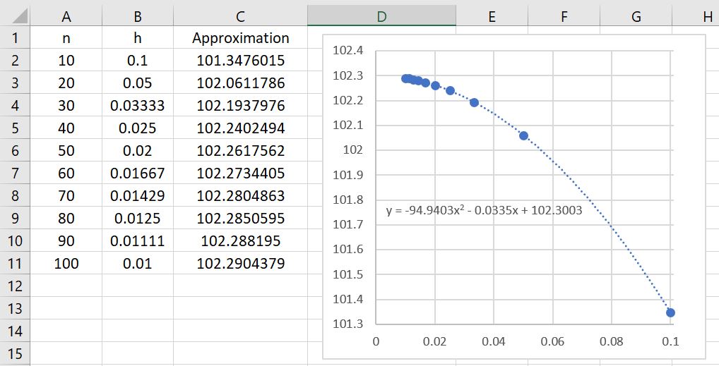
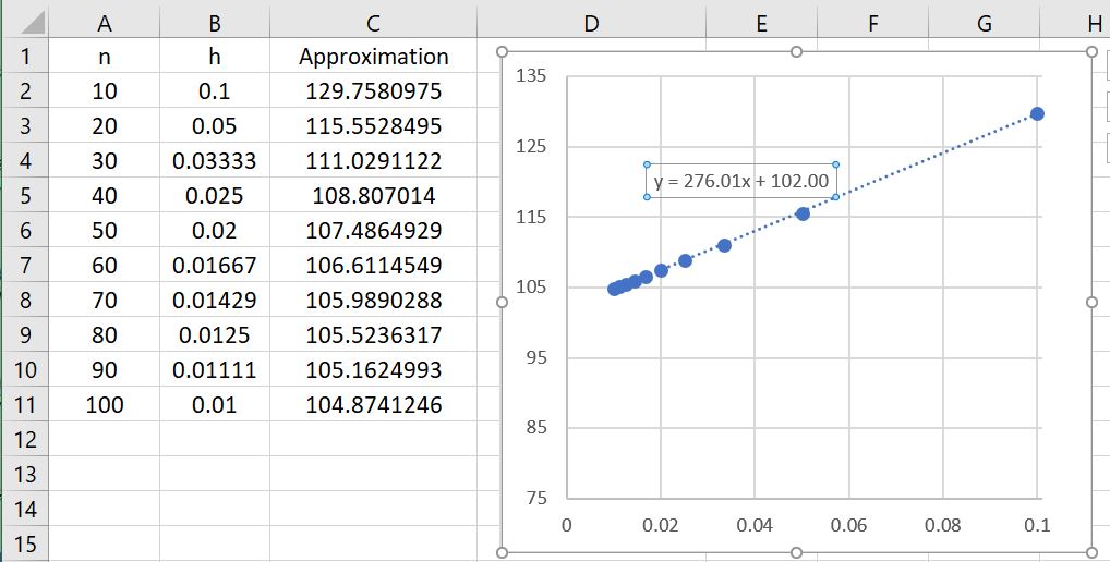
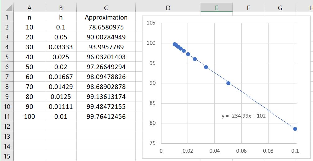
 for different numbers of subintervals. If we take
  and
and  , then the error should be approximately equal to

 .
.
 , so that the error becomes

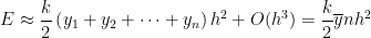
 is the average of the
  . Clearly, this average is somewhere between the smallest and the largest of the . Since
  is a continuous function, that means that there must be some value of
  between
  and
and  — and therefore between
  and
and  — so that
  by the Intermediate Value Theorem. We conclude that the error can be written as
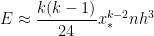
is the length of one subinterval, we see that  is the total length of the interval
 ![[a,b]](https://s0.wp.com/latex.php?latex=%5Ba%2Cb%5D&bg=ffffff&fg=000000&s=0&c=20201002) . Therefore,
. Therefore,
 is determined by , , and
  . In other words, for the special case , we have established that the error from the Midpoint Rule is approximately quadratic in — without resorting to the generalized mean-value theorem and confirming the numerical observations we made earlier.
 .
. will be the sum of the errors for the integrals over
  .
. ,
, .
.
 , so that the error becomes
 ,
, is the average of the
  is a continuous function, that means that there must be some value of
  and
and  — and therefore between
  by the Intermediate Value Theorem. We conclude that the error can be written as
 ,
, ,
,
![\int_a^b f(x) \, dx \approx h \left[f(x_1) + f(x_2) + \dots + f(x_n) \right] \equiv R_n](https://s0.wp.com/latex.php?latex=%5Cint_a%5Eb+f%28x%29+%5C%2C+dx+%5Capprox+h+%5Cleft%5Bf%28x_1%29+%2B+f%28x_2%29+%2B+%5Cdots+%2B+f%28x_n%29+%5Cright%5D+%5Cequiv+R_n&bg=ffffff&fg=000000&s=0&c=20201002)

![= \displaystyle \frac{1}{k+1} \left[x_i^{k+1} + {k+1 \choose 1} x_i^k h + {k+1 \choose 2} x_i^{k-1} h^2 + O(h^3) - x_i^{k+1} \right]](https://s0.wp.com/latex.php?latex=%3D+%5Cdisplaystyle+%5Cfrac%7B1%7D%7Bk%2B1%7D+%5Cleft%5Bx_i%5E%7Bk%2B1%7D+%2B+%7Bk%2B1+%5Cchoose+1%7D+x_i%5Ek+h+%2B+%7Bk%2B1+%5Cchoose+2%7D+x_i%5E%7Bk-1%7D+h%5E2+%2B+O%28h%5E3%29+-+x_i%5E%7Bk%2B1%7D+%5Cright%5D&bg=ffffff&fg=000000&s=0&c=20201002)
![= \displaystyle \frac{1}{k+1} \left[ (k+1) x_i^k h + \frac{(k+1)k}{2} x_i^{k-1} h^2 + O(h^3) \right]](https://s0.wp.com/latex.php?latex=%3D+%5Cdisplaystyle+%5Cfrac%7B1%7D%7Bk%2B1%7D+%5Cleft%5B+%28k%2B1%29+x_i%5Ek+h+%2B+%5Cfrac%7B%28k%2B1%29k%7D%7B2%7D+x_i%5E%7Bk-1%7D+h%5E2+%2B+O%28h%5E3%29+%5Cright%5D&bg=ffffff&fg=000000&s=0&c=20201002)

 can be formally defined, but here we’ll just take it to mean “terms that have a factor of
  and thus can be safely ignored.
 .
.
![[x_i, x_i+h]](https://s0.wp.com/latex.php?latex=%5Bx_i%2C+x_i%2Bh%5D&bg=ffffff&fg=000000&s=0&c=20201002) , which is proportional to
, which is proportional to  , generates a total error on


 .
. ,
, .
.
 ,
, — and therefore between
 ![\int_a^b f(x) \, dx \approx h \left[f(x_0) + f(x_1) + \dots + f(x_{n-1}) \right] \equiv L_n](https://s0.wp.com/latex.php?latex=%5Cint_a%5Eb+f%28x%29+%5C%2C+dx+%5Capprox+h+%5Cleft%5Bf%28x_0%29+%2B+f%28x_1%29+%2B+%5Cdots+%2B+f%28x_%7Bn-1%7D%29+%5Cright%5D+%5Cequiv+L_n&bg=ffffff&fg=000000&s=0&c=20201002)

 and
and  — is approximately linear in