I’m using the Twelve Days of Christmas (and perhaps a few extra days besides) to do something that I should have done a long time ago: collect past series of posts into a single, easy-to-reference post. The following posts formed my series on different techniques that I’ll use to try to convince students that .
Part 1: Converting the decimal expansion to a fraction, with algebra.
I’m doing something that I should have done a long time ago: collect past series of posts into a single, easy-to-reference post. The following posts formed my series on how I remind students about Taylor series. I often use this series in a class like Differential Equations, when Taylor series are needed but my class has simply forgotten about what a Taylor series is and why it’s important.
Part 1: Introduction – Why a Taylor series is important, and different applications of Taylor series.
Part 2: How I get students to understand the finite Taylor polynomial by solving a simple initial-value problem.
Part 3: Making the jump to an infinite series, and issues about tests of convergence.
Part 4: Application to , and a numerical investigation of speed of convergence.
Part 5: Application to and other related functions, including and .
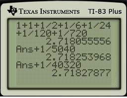
In yesterday’s post, I showed that using the original definition (in terms of an area under a hyperbola) does not lend itself well to numerically approximating . Let’s now look at the other two methods.
2. The limit gives a somewhat more tractable way of approximating , at least with a modern calculator. However, you can probably imagine the fun of trying to use this formula without a calculator.
3. The best way to compute (or, in general, ) is with Taylor series. The fractions get very small very quickly, leading to rapid convergence. Indeed, with only terms up to , this approximation beats the above approximation with . Adding just two extra terms comes close to matching the accuracy of the above limit when .
More about approximating via Taylor series can be found in my previous post.
In this series of posts, I explore properties of complex numbers that explain some surprising answers to exponential and logarithmic problems using a calculator (see video at the bottom of this post). These posts form the basis for a sequence of lectures given to my future secondary teachers.
To begin, we recall that the trigonometric form of a complex number is
where and , with in the appropriate quadrant. As noted before, this is analogous to converting from rectangular coordinates to polar coordinates.
There’s a shorthand notation for the right-hand side () that, at long last, I will explain in today’s post.
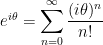
Definition. If is a complex number, then we define
This of course matches the Taylor expansion of for real numbers .
This theorem explains one of the calculator’s results:
.
That said, you can imagine that finding something like would be next to impossible by directly plugging into the series and trying to simply the answer. The good news is that there’s an easy way to compute for complex numbers , which we develop in the next few posts.
For completeness, here’s the movie that I use to engage my students when I begin this sequence of lectures.
In this series of posts, I explore properties of complex numbers that explain some surprising answers to exponential and logarithmic problems using a calculator (see video at the bottom of this post). These posts form the basis for a sequence of lectures given to my future secondary teachers.
Definition. If is a complex number, then we define
Even though this isn’t the usual way of defining the exponential function for real numbers, the good news is that one Law of Exponents remains true. (At we saw in an earlier post in this series, we can’t always assume that the usual Laws of Exponents will remain true when we permit the use of complex numbers.)
Theorem. If and are complex numbers, then .
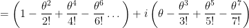
I will formally prove this in the next post. Today, I want to talk about the idea behind the proof. Notice that
Let’s multiply this out (ugh!), but we’ll only worry about terms where the sum of the exponents of and is 4 or less. Here we go…
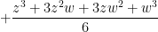
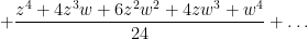
Next, we rearrange the terms according to the sum of the exponents. For example, the terms with , , , and are placed together because the sum of the exponents for each of these terms is 3.
For each line, we obtain a common denominator:
We recognize the familiar entries of Pascal’s triangle in the coefficients of the numerators, and so it appears that
If the pattern on the right-hand side holds up for exponents greater than 4, this proves that .
So that’s the idea of the proof. The formal proof will be presented in the next post.
For completeness, here’s the movie that I use to engage my students when I begin this sequence of lectures.
After class one day, a student approached me with an interesting question:
Is there an easy function without an easy Taylor expansion?
This question really struck me for several reasons.
Most functions do not have an easy Taylor (or Maclaurin) expansion. After all, the formula for a Taylor expansion involves the th derivative of the original function, and higher-order derivatives usually get progressively messier with each successive differentiation.
Most of the series expansions that are taught in Calculus II arise from functions that somehow violate the above rule, like , , , and .
Therefore, this student was under the misconception that most easy functions have easy Taylor expansions, while in reality most functions do not.
It took me a moment to answer his question, but I answered with . Successively using the Quotient Rule makes the derivatives of messier and messier, but definitely qualifies as an easy function that most students have seen since high school. It turns out that the Taylor expansion of can be written as an infinite series using the Bernoulli numbers, but that’s a concept that most calculus students haven’t seen yet.
Every once in a while, I’ll give a “fun lecture” to my students. The rules of a “fun lecture” are that I talk about some advanced applications of classroom topics, but I won’t hold them responsible for these ideas on homework and on exams. In other words, they can just enjoy the lecture without being responsible for its content.
This series of posts describes a fun lecture that I’ve given to my Precalculus students after they’ve learned about partial fractions and geometric series.
In the 1949 cartoon “Hare Do,” Bugs Bunny comes across the following sign when trying to buy candy (well, actually, a carrot) from a vending machine. The picture below can be seen at the 2:40 mark of this video: http://www.ulozto.net/live/xSG8zto/bugs-bunny-hare-do-1949-avi
How many ways are there of expressing 20 cents using pennies, nickels, dimes, and (though not applicable to this problem) quarters? Believe it or not, this is equivalent to the following very complicated multiplication problem:
On the first line, the exponents are all multiples of 1. On the second line, the exponents are all multiples of 5. On the third line, the exponents are all multiples of 10. On the fourth line, the exponents are all multiples of 25.
How many ways are there of constructing a product of from the product of these four infinite series? I offer a thought bubble if you’d like to think about it before seeing the answer.
There are actually 9 ways. We could choose from the first, second, and fourth lines while choosing from the third line. So,
There are 8 other ways. For each of these lines, the first term comes from the first infinite series, the second term comes from the second infinite series, and so on.
The nice thing is that each of these expressions is conceptually equivalent to a way of expressing 20 cents using pennies, nickels, dimes, and quarters. In each case, the value in parentheses matches an exponent.
Notice that the last line didn’t appear in the Bugs Bunny cartoon.
Using the formula for an infinite geometric series (and assuming ), we may write the infinite product as
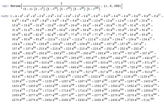
When written as an infinite series — that is, as a Taylor series about — the coefficients provide the number of ways of expressing that many cents using pennies, nickels, dimes and quarters. This Taylor series can be computed with Mathematica:
Looking at the coefficient of , we see that there are indeed 9 ways of expressing 20 cents with pennies, nickels, dimes, and quarters. We also see that there are 242 of expressing 1 dollar and 1463 ways of expressing 2 dollars.
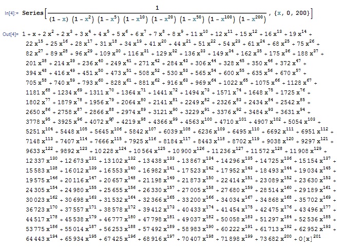
The United States also has 50-cent coins and dollar coins, although they are rarely used in circulation. Our answers become slightly different if we permit the use of these larger coins:
Finally, just for the fun of it, the coins in the United Kingdom are worth 1 pence, 2 pence, 5 pence, 10 pence, 20 pence, 50 pence, 100 pence (1 pound), and 200 pence (2 pounds). With these different coins, there are 41 ways of expressing 20 pence, 4563 ways of expressing 1 pound, and 73,682 ways of expressing 2 pounds.
For more discussion about this application of generating functions — including ways of determining the above coefficients without Mathematica — I’ll refer to the 1000+ results of the following Google search:
Many math majors don’t have immediate recall of the formula for an infinite geometric series. They often can remember that there is a formula, but they can’t recollect the details. While it’s I think it’s OK that they don’t have the formula memorized, I think is a real shame that they’re also unaware of where the formula comes from and hence are unable to rederive the formula if they’ve forgotten it.
In this post, I’d like to give some thoughts about why the formula for an infinite geometric series is important for other areas of mathematics besides Precalculus. (There may be others, but here’s what I can think of in one sitting.)
1. An infinite geometric series is actually a special case of a Taylor series. (See https://meangreenmath.com/2013/07/05/reminding-students-about-taylor-series-part-5/ for details.) Therefore, it would be wonderful if students learning Taylor series in Calculus II could be able to relate the new topic (Taylor series) to their previous knowledge (infinite geometric series) which they had already seen in Precalculus.
2. An infinite geometric series is also a special case of the binomial series , when does not have to be a positive integer and hence Pascal’s triangle cannot be used to find the expansion.
3. Infinite geometric series is a rare case when an infinite sum can be found exactly. In Calculus II, a whole battery of tests (e.g., the Root Test, the Ratio Test, the Limit Comparison Test) are introduced to determine whether a series converges or not. In other words, these tests only determine if an answer exists, without determining what the answer actually is.
Throughout the entire undergraduate curriculum, I’m aware of only four types of series that can actually be evaluated exactly.
An infinite geometric series with
The Taylor series of a real analytic function. (Of course, an infinite geometric series is a special case of a Taylor series.)
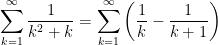
A telescoping series. For example, using partial fractions and cancelling a bunch of terms, we find that
An infinite series that arises from Parseval’s theorem in Fourier analysis.
4. Infinite geometric series are essential for proving basic facts about decimal representations that we often take for granted.
5. Properties of an infinite geometric series are needed to find the mean and standard deviation of a geometric random variable, which is used to predict the number of independent trials needed before an event happens. This is used for analyzing the coupon collector’s problem, among other applications.
This is the fifth in a series of posts about calculating roots without a calculator, with special consideration to how these tales can engage students more deeply with the secondary mathematics curriculum. As most students today have a hard time believing that square roots can be computed without a calculator, hopefully giving them some appreciation for their elders.
Today’s story takes us back to a time before the advent of cheap pocket calculators: 1949.
The following story comes from the chapter “Lucky Numbers” of Surely You’re Joking, Mr. Feynman!, a collection of tales by the late Nobel Prize winning physicist, Richard P. Feynman. Feynman was arguably the greatest American-born physicist — the subject of the excellent biography Genius: The Life and Science of Richard Feynman — and he had a tendency to one-up anyone who tried to one-up him. (He was also a serial philanderer, but that’s another story.) Here’s a story involving how, in the summer of 1949, he calculated without a calculator.
The first time I was in Brazil I was eating a noon meal at I don’t know what time — I was always in the restaurants at the wrong time — and I was the only customer in the place. I was eating rice with steak (which I loved), and there were about four waiters standing around.
A Japanese man came into the restaurant. I had seen him before, wandering around; he was trying to sell abacuses. (Note: At the time of this story, before the advent of pocket calculators, the abacus was arguably the world’s most powerful hand-held computational device.) He started to talk to the waiters, and challenged them: He said he could add numbers faster than any of them could do.
The waiters didn’t want to lose face, so they said, “Yeah, yeah. Why don’t you go over and challenge the customer over there?”
The man came over. I protested, “But I don’t speak Portuguese well!”
The waiters laughed. “The numbers are easy,” they said.
They brought me a paper and pencil.
The man asked a waiter to call out some numbers to add. He beat me hollow, because while I was writing the numbers down, he was already adding them as he went along.
I suggested that the waiter write down two identical lists of numbers and hand them to us at the same time. It didn’t make much difference. He still beat me by quite a bit.
However, the man got a little bit excited: he wanted to prove himself some more. “Multiplição!” he said.
Somebody wrote down a problem. He beat me again, but not by much, because I’m pretty good at products.
The man then made a mistake: he proposed we go on to division. What he didn’t realize was, the harder the problem, the better chance I had.
We both did a long division problem. It was a tie.
This bothered the hell out of the Japanese man, because he was apparently well trained on the abacus, and here he was almost beaten by this customer in a restaurant.
“Raios cubicos!” he says with a vengeance. Cube roots! He wants to do cube roots by arithmetic. It’s hard to find a more difficult fundamental problem in arithmetic. It must have been his topnotch exercise in abacus-land.
He writes down a number on some paper— any old number— and I still remember it: . He starts working on it, mumbling and grumbling: “Mmmmmmagmmmmbrrr”— he’s working like a demon! He’s poring away, doing this cube root.
Meanwhile I’m just sitting there.
One of the waiters says, “What are you doing?”.
I point to my head. “Thinking!” I say. I write down on the paper. After a little while I’ve got .
The man with the abacus wipes the sweat off his forehead: “Twelve!” he says.
“Oh, no!” I say. “More digits! More digits!” I know that in taking a cube root by arithmetic, each new digit is even more work that the one before. It’s a hard job.
He buries himself again, grunting “Rrrrgrrrrmmmmmm …,” while I add on two more digits. He finally lifts his head to say, “!”
The waiter are all excited and happy. They tell the man, “Look! He does it only by thinking, and you need an abacus! He’s got more digits!”
He was completely washed out, and left, humiliated. The waiters congratulated each other.
How did the customer beat the abacus?
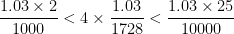
The number was . I happened to know that a cubic foot contains cubic inches, so the answer is a tiny bit more than . The excess, , is only one part in nearly , and I had learned in calculus that for small fractions, the cube root’s excess is one-third of the number’s excess. So all I had to do is find the fraction , and multiply by (divide by and multiply by ). So I was able to pull out a whole lot of digits that way.
A few weeks later, the man came into the cocktail lounge of the hotel I was staying at. He recognized me and came over. “Tell me,” he said, “how were you able to do that cube-root problem so fast?”
I started to explain that it was an approximate method, and had to do with the percentage of error. “Suppose you had given me . Now the cube root of is …”
He picks up his abacus: zzzzzzzzzzzzzzz— “Oh yes,” he says.
I realized something: he doesn’t know numbers. With the abacus, you don’t have to memorize a lot of arithmetic combinations; all you have to do is to learn to push the little beads up and down. You don’t have to memorize 9+7=16; you just know that when you add 9, you push a ten’s bead up and pull a one’s bead down. So we’re slower at basic arithmetic, but we know numbers.
Furthermore, the whole idea of an approximate method was beyond him, even though a cubic root often cannot be computed exactly by any method. So I never could teach him how I did cube roots or explain how lucky I was that he happened to choose .
The key part of the story, “for small fractions, the cube root’s excess is one-third of the number’s excess,” deserves some elaboration, especially since this computational trick isn’t often taught in those terms anymore. If , then , so that . Since , the equation of the tangent line to at is
.
The key observation is that, for , the graph of will be very close indeed to the graph of . In Calculus I, this is sometimes called the linearization of at . In Calculus II, we observe that these are the first two terms in the Taylor series expansion of about .
For Feynman’s problem, , so that if $x \approx 0$. Then $\latex \sqrt[3]{1729.03}$ can be rewritten as
This last equation explains the line “all I had to do is find the fraction , and multiply by .” With enough patience, the first few digits of the correction can be mentally computed since
So Feynman could determine quickly that the answer was .
By the way,
So the linearization provides an estimate accurate to eight significant digits. Additional digits could be obtained by using the next term in the Taylor series.
I have a similar story to tell. Back in 1996 or 1997, when I first moved to Texas and was making new friends, I quickly discovered that one way to get odd facial expressions out of strangers was by mentioning that I was a math professor. Occasionally, however, someone would test me to see if I really was a math professor. One guy (who is now a good friend; later, we played in the infield together on our church-league softball team) asked me to figure out without a calculator — before someone could walk to the next room and return with the calculator. After two seconds of panic, I realized that I was really lucky that he happened to pick a number close to . Using the same logic as above,
.
Knowing that this came from a linearization and that the tangent line to lies above the curve, I knew that this estimate was too high. But I didn’t have time to work out a correction (besides, I couldn’t remember the full Taylor series off the top of my head), so I answered/guessed , hoping that I did the arithmetic correctly. You can imagine the amazement when someone punched into the calculator to get
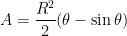
Is calculus really necessary for obtaining a Taylor series? Years ago, while perusing an old Schaum’s outline, I found a very curious formula for the area of a circular segment:
The thought occurred to me that was the first term in the Taylor series expansion of about , and perhaps there was a way to use this picture to generate the remaining terms of the Taylor series.
This insight led to a paper which was published in College Mathematics Journal: cmj38-1-058-059. To my surprise and delight, this paper was later selected for inclusion in The Calculus Collection: A Resource for AP and Beyond, which is a collection of articles from the publications of Mathematical Association of America specifically targeted toward teachers of AP Calculus.
Although not included in the article, it can be proven that this iterative method does indeed yield the successive Taylor polynomials of , adding one extra term with each successive step.
I carefully scaffolded these steps into a project that I twice assigned to my TAMS precalculus students. Both semesters, my students got it… and they were impressed to know the formula that their calculators use to compute . So I think this project is entirely within the grasp of precocious precalculus students.
I personally don’t know of a straightforward way of obtaining the expansion of without calculus. However, once the expansion of is known, the expansion of can be surmised without calculus. To do this, we note that
Truncating the series after terms and squaring — and being very careful with the necessary simplifications — yield the first terms in the Taylor series of .


 , and a numerical investigation of speed of convergence.
 and other related functions, including
  and
and  .
. and
and  , and Euler’s formula.
 can be thought about in three different ways.
 .
. 2. We have the limits
 .
. . From this derivative,
  about
about  can be computed:
 to find

 gives a somewhat more tractable way of approximating
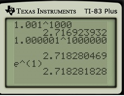
 get very small very quickly, leading to rapid convergence. Indeed, with only terms up to
  , this approximation beats the above approximation with
  . Adding just two extra terms comes close to matching the accuracy of the above limit when
  .
.
 is
is
 and
and  , with
  in the appropriate quadrant. As noted before, this is analogous to converting from rectangular coordinates to polar coordinates.
 ) that, at long last, I will explain in today’s post.
 is a complex number, then we define
 .
. .
.

 ,
, .
. would be next to impossible by directly plugging into the series and trying to simply the answer. The good news is that there’s an easy way to compute
  for complex numbers
 are complex numbers, then
  .
.


 ,
,  ,
,  , and
, and  are placed together because the sum of the exponents for each of these terms is 3.


 th derivative of the original function, and higher-order derivatives usually get progressively messier with each successive differentiation.
 .
. .
.  messier and messier, but
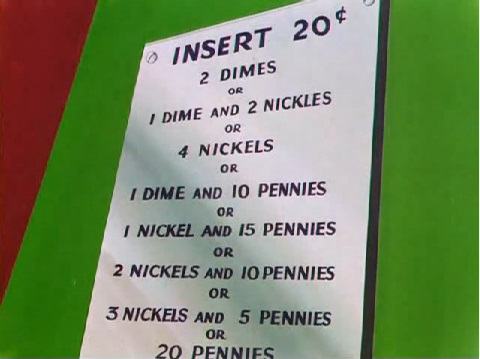
![\left[1 + x + x^2 + x^3 + x^4 + x^5 + \dots \right]](https://s0.wp.com/latex.php?latex=%5Cleft%5B1+%2B+x+%2B+x%5E2+%2B+x%5E3+%2B+x%5E4+%2B+x%5E5+%2B+%5Cdots+%5Cright%5D&bg=ffffff&fg=000000&s=0&c=20201002)
![\times \left[1 + x^5 + x^{10} + x^{15} + x^{20} + x^{25} + \dots \right]](https://s0.wp.com/latex.php?latex=%5Ctimes+%5Cleft%5B1+%2B+x%5E5+%2B+x%5E%7B10%7D+%2B+x%5E%7B15%7D+%2B+x%5E%7B20%7D+%2B+x%5E%7B25%7D+%2B+%5Cdots+%5Cright%5D&bg=ffffff&fg=000000&s=0&c=20201002)
![\times \left[1 + x^{10} + x^{20} + x^{30} + x^{40} + x^{50} + \dots \right]](https://s0.wp.com/latex.php?latex=%5Ctimes+%5Cleft%5B1+%2B+x%5E%7B10%7D+%2B+x%5E%7B20%7D+%2B+x%5E%7B30%7D+%2B+x%5E%7B40%7D+%2B+x%5E%7B50%7D+%2B+%5Cdots+%5Cright%5D&bg=ffffff&fg=000000&s=0&c=20201002)
![\times \left[1 + x^{25} + x^{50} + x^{75} + x^{100} + x^{125} + \dots \right]](https://s0.wp.com/latex.php?latex=%5Ctimes+%5Cleft%5B1+%2B+x%5E%7B25%7D+%2B+x%5E%7B50%7D+%2B+x%5E%7B75%7D+%2B+x%5E%7B100%7D+%2B+x%5E%7B125%7D+%2B+%5Cdots+%5Cright%5D&bg=ffffff&fg=000000&s=0&c=20201002)
 from the product of these four infinite series? I offer a thought bubble if you’d like to think about it before seeing the answer.


 : 15 pennies (15 cents) and 1 nickel (5 cents)
 ), we may write the infinite product as
 — the coefficients provide the number of ways of expressing that many cents using pennies, nickels, dimes and quarters. This Taylor series can be computed with Mathematica:
 , when


 . See
. See  actually converges and must correspond to a real number. See
  must have a repeating block of length
  which contains the digits of
  . See
. See ![\sqrt[3]{1729.03}](https://s0.wp.com/latex.php?latex=%5Csqrt%5B3%5D%7B1729.03%7D&bg=ffffff&fg=000000&s=0&c=20201002) without a calculator.
without a calculator. . He starts working on it, mumbling and grumbling: “Mmmmmmagmmmmbrrr”— he’s working like a demon! He’s poring away, doing this cube root.
 on the paper. After a little while I’ve got
  .
. !”
!” cubic inches, so the answer is a tiny bit more than
  , is only one part in nearly
  , and I had learned in calculus that for small fractions, the cube root’s excess is one-third of the number’s excess. So all I had to do is find the fraction
  , and multiply by
  (divide by
  and multiply by
  . Now the cube root of
  is
is  , then
  , so that
  . Since
  , the equation of the tangent line to
  at
at  .
. , the graph of
  will be very close indeed to the graph of
  at
at  . In Calculus II, we observe that these are the first two terms in the
  .
. , so that
 ![\sqrt[3]{1+x} \approx 1 + \frac{1}{3} x](https://s0.wp.com/latex.php?latex=%5Csqrt%5B3%5D%7B1%2Bx%7D+%5Capprox+1+%2B+%5Cfrac%7B1%7D%7B3%7D+x&bg=ffffff&fg=000000&s=0&c=20201002) if $x \approx 0$. Then $\latex \sqrt[3]{1729.03}$ can be rewritten as
if $x \approx 0$. Then $\latex \sqrt[3]{1729.03}$ can be rewritten as![\sqrt[3]{1729.03} = \sqrt[3]{1728} \sqrt[3]{ \displaystyle \frac{1729.03}{1728} }](https://s0.wp.com/latex.php?latex=%5Csqrt%5B3%5D%7B1729.03%7D+%3D+%5Csqrt%5B3%5D%7B1728%7D+%5Csqrt%5B3%5D%7B+%5Cdisplaystyle+%5Cfrac%7B1729.03%7D%7B1728%7D+%7D&bg=ffffff&fg=000000&s=0&c=20201002)
![\sqrt[3]{1729.03} = 12 \sqrt[3]{\displaystyle 1 + \frac{1.03}{1728}}](https://s0.wp.com/latex.php?latex=%5Csqrt%5B3%5D%7B1729.03%7D+%3D+12+%5Csqrt%5B3%5D%7B%5Cdisplaystyle+1+%2B+%5Cfrac%7B1.03%7D%7B1728%7D%7D&bg=ffffff&fg=000000&s=0&c=20201002)
![\sqrt[3]{1729.03} \approx 12 \left( 1 + \displaystyle \frac{1}{3} \times \frac{1.03}{1728} \right)](https://s0.wp.com/latex.php?latex=%5Csqrt%5B3%5D%7B1729.03%7D+%5Capprox+12+%5Cleft%28+1+%2B+%5Cdisplaystyle+%5Cfrac%7B1%7D%7B3%7D+%5Ctimes+%5Cfrac%7B1.03%7D%7B1728%7D+%5Cright%29&bg=ffffff&fg=000000&s=0&c=20201002)
![\sqrt[3]{1729.03} \approx 12 + 4 \times \displaystyle \frac{1.03}{1728}](https://s0.wp.com/latex.php?latex=%5Csqrt%5B3%5D%7B1729.03%7D+%5Capprox+12+%2B+4+%5Ctimes+%5Cdisplaystyle+%5Cfrac%7B1.03%7D%7B1728%7D&bg=ffffff&fg=000000&s=0&c=20201002)


 .
.![\sqrt[3]{1729.03} \approx 12.00238378\dots](https://s0.wp.com/latex.php?latex=%5Csqrt%5B3%5D%7B1729.03%7D+%5Capprox+12.00238378%5Cdots&bg=ffffff&fg=000000&s=0&c=20201002)

 without a calculator — before someone could walk to the next room and return with the calculator. After two seconds of panic, I realized that I was really lucky that he happened to pick a number close to
  . Using the same logic as above,
 .
. lies above the curve, I knew that this estimate was too high. But I didn’t have time to work out a correction (besides, I couldn’t remember the full Taylor series off the top of my head), so I answered/guessed
  , hoping that I did the arithmetic correctly. You can imagine the amazement when someone punched into the calculator to get

 about
about  , and perhaps there was a way to use this picture to generate the remaining terms of the Taylor series.
 without calculus. However, once the expansion of