I conclude this series of posts with thoughts about infinite series which use reciprocals of positive integers. I offer this post for the enrichment of talented Precalculus students who have exhibited mastery of geometric series.
Geometric. As we’ve discussed at length, the series

converges and is in fact equal to  .
.
Harmonic. Including the reciprocals of all positive integers is called a harmonic series:
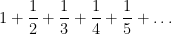
As shown in the link to the MathWorld website, this series actually diverges, even though the terms get smaller and smaller.
So we’ve made an observation: if too many reciprocals are included, the series diverges. But if we take enough of them away, then we can still end up with a series that is infinite but converges.
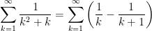
Squares. Let’s now consider the reciprocals of perfect squares:
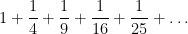
Clearly, we’ve taken away a lot of the terms of the harmonic series? Have we taken enough away so that the series converges? It turns out that the answer is yes. And the answer is precisely what you’d think it should be (not):  . This is just another way that the circumference of a circle has an odd way of appearing in the most unexpected of places.
The proof that this series equals requires the clever use of Parseval’s theorem from Fourier analysis.
Fourth Powers. Let’s now turn to the reciprocals of fourth powers:

By the Direct Comparison Test and the series for reciprocals of squares, this series converges. Using Parseval’s theorem, it can be shown that the answer is  .
.
Cubes. Now let’s investigate the reciprocals of cubes:
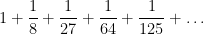
Again by the Direct Comparison Test and the series for reciprocals for squares, this series must converge. This sum is called Apéry’s constant. However, and amazingly, no one knows what the answer is. Of course, a computer can be programmed to evaluate this series to as many decimal places as desired. According to Wikipedia, this sum was evaluated to over 100 billion decimal places in 2010. However, to the best of my knowledge, no one has figured out if there’s a simple way of writing the answer, like or .
So if you figure out a simple way to evaluate Apéry’s constant, feel free to call me collect.
The previous four series are example of Riemann’s zeta function, which is of central importance in number theory and is the focus of the celebrated Riemann Hypothesis, for which a solution is worth a cool $1 million.
Primes. Now let’s consider the reciprocals of primes:

As noted above, the harmonic series diverges, but if we remove enough terms from the harmonic series, then it’s possible to make an infinite series that converges. So the central question is, did we remove enough fractions (by taking away all of the composite denominators) so that the series converges?
Surprisingly, the answer is no: the sum of the reciprocals of the primes actually diverges. The proof actually requires a graduate-level class in analytic number theory.

By no means would I expect high school students to master all of the above facts. As noted above, the subject of this post is mostly for the enrichment of high school students who have mastered infinite geometric series.
That said, students who know the following facts from Precalculus will be well-served when they reach calculus and other university-level mathematics courses.
- They should either know the formula for an infinite geometric series or else be able to quickly derive it.
- They should know that not every infinite geometric series is geometric.
- They should know that not every infinite series converges.
- They should be familiar with the meaning of the terms converge and diverge.


![= e^{w [\ln r + i \theta]}](https://s0.wp.com/latex.php?latex=%3D+e%5E%7Bw+%5B%5Cln+r+%2B+i+%5Ctheta%5D%7D&bg=ffffff&fg=000000&s=0&c=20201002)


 . For the base of
  , we note that
 .
. ,
, . To begin,
 .
.


![= e^{-\pi} (\cos [\ln 8] + i \sin [ \ln 8 ] )](https://s0.wp.com/latex.php?latex=%3D+e%5E%7B-%5Cpi%7D+%28%5Ccos+%5B%5Cln+8%5D+%2B+i+%5Csin+%5B+%5Cln+8+%5D+%29&bg=ffffff&fg=000000&s=0&c=20201002)

 , and
, and  in the case that
  . However, this complex logarithm doesn’t always work the way you’d think it work. For example,
 .
.
 .
.![\log \left[ (-1) \cdot (-1) \right] = \log 1 = 0](https://s0.wp.com/latex.php?latex=%5Clog+%5Cleft%5B+%28-1%29+%5Ccdot+%28-1%29+%5Cright%5D+%3D+%5Clog+1+%3D+0&bg=ffffff&fg=000000&s=0&c=20201002) ,
, .
. ,
, .
.![(-\pi,\pi]](https://s0.wp.com/latex.php?latex=%28-%5Cpi%2C%5Cpi%5D&bg=ffffff&fg=000000&s=0&c=20201002) leads to the definition of the complex logarithm.
leads to the definition of the complex logarithm.
 .
. is usually dedicated to base 10. However, in higher-level mathematics courses,
  , but
, but  requires a little more thought. But nearly all major theorems that involve logarithms specifically employ natural logarithms. Indeed, when I first become a professor, I had to remind myself that my students used
  for natural logarithms and not
  for base-10 logarithms and not
  is entered, it assumes that a real answer is expected, and so the calculatore returns an error message. On the other hand, when
  is entered, it assumes that the user wants the principal complex logarithm. Since
  , the calculator correctly returns
  as the answer. (Of course, the calculator still uses
  .
. , then
 and that the angle
  radians. In other words,
 and
and  for any integer
  .
. .
. . This could have been any nonzero number, including complex numbers, and there still would have been an infinite number of solutions. (This is completely analogous to solving a trigonometric equation like
  , which similarly has an infinite number of solutions.) For example, the complex solutions of the equation
 is
is  .
. .
.
 for real numbers
  .
.
 to a power and get a negative number. Obviously, this is impossible when using only real numbers.
 .
.
 axis represents the values of
  and the
  axis represents the values of
  . In other words, we start with
  and add all the terms on the line
  (i.e., the
  and then add all the terms on the next horizontal line. And so on.
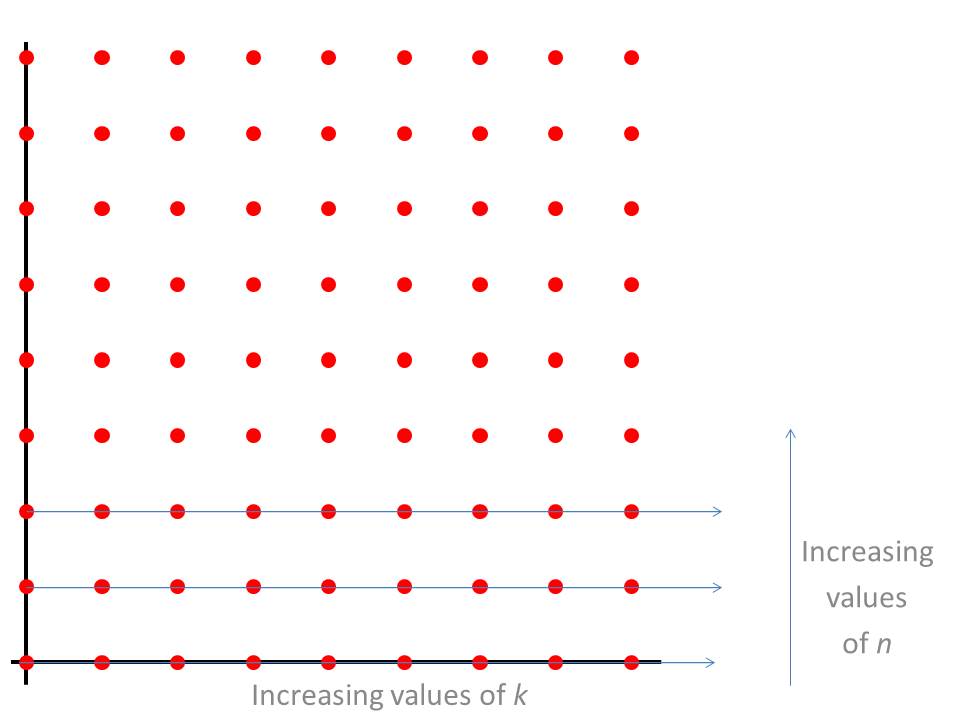
 . Then for a fixed value of
  , the values of
 gets replaced by
  . Since
  , we have
 terms to this expression for reasons that will become clear shortly:

 is a binomial coefficent:
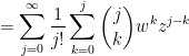

 , using the dummy variable
  ,
,
 , when


 . See
. See  actually converges and must correspond to a real number. See
  must have a repeating block of length
  . See
. See 