Numerical integration is a standard topic in first-semester calculus. From time to time, I have received questions from students on various aspects of this topic, including:
- Why is numerical integration necessary in the first place?
- Where do these formulas come from (especially Simpson’s Rule)?
- How can I do all of these formulas quickly?
- Is there a reason why the Midpoint Rule is better than the Trapezoid Rule?
- Is there a reason why both the Midpoint Rule and the Trapezoid Rule converge quadratically?
- Is there a reason why Simpson’s Rule converges like the fourth power of the number of subintervals?
In this series, I hope to answer these questions. While these are standard questions in a introductory college course in numerical analysis, and full and rigorous proofs can be found on Wikipedia and Mathworld, I will approach these questions from the point of view of a bright student who is currently enrolled in calculus and hasn’t yet taken real analysis or numerical analysis.

In the previous post in this series, I discussed three different ways of numerically approximating the definite integral 


In this series, we’ll choose equal-sized subintervals of the interval ![[a,b]](https://s0.wp.com/latex.php?latex=%5Ba%2Cb%5D&bg=ffffff&fg=000000&s=0&c=20201002)


![\int_a^b f(x) \, dx \approx h \left[f(x_0) + f(x_1) + \dots + f(x_{n-1}) \right] \equiv L_n](https://s0.wp.com/latex.php?latex=%5Cint_a%5Eb+f%28x%29+%5C%2C+dx+%5Capprox+h+%5Cleft%5Bf%28x_0%29+%2B+f%28x_1%29+%2B+%5Cdots+%2B+f%28x_%7Bn-1%7D%29+%5Cright%5D+%5Cequiv+L_n&bg=ffffff&fg=000000&s=0&c=20201002)
using left endpoints,
![\int_a^b f(x) \, dx \approx h \left[f(x_1) + f(x_2) + \dots + f(x_n) \right] \equiv R_n](https://s0.wp.com/latex.php?latex=%5Cint_a%5Eb+f%28x%29+%5C%2C+dx+%5Capprox+h+%5Cleft%5Bf%28x_1%29+%2B+f%28x_2%29+%2B+%5Cdots+%2B+f%28x_n%29+%5Cright%5D+%5Cequiv+R_n&bg=ffffff&fg=000000&s=0&c=20201002)
using right endpoints, and
![\int_a^b f(x) \, dx \approx h \left[f(c_1) + f(c_2) + \dots + f(c_n) \right] \equiv M_n](https://s0.wp.com/latex.php?latex=%5Cint_a%5Eb+f%28x%29+%5C%2C+dx+%5Capprox+h+%5Cleft%5Bf%28c_1%29+%2B+f%28c_2%29+%2B+%5Cdots+%2B+f%28c_n%29+%5Cright%5D+%5Cequiv+M_n&bg=ffffff&fg=000000&s=0&c=20201002)
using the midpoints of the subintervals. We have also derived the Trapezoid Rule
![\int_a^b f(x) \, dx \approx \displaystyle \frac{h}{2} [f(x_0) + 2f(x_1) + \dots + 2f(x_{n-1}) + f(x_n)] \equiv T_n](https://s0.wp.com/latex.php?latex=%5Cint_a%5Eb+f%28x%29+%5C%2C+dx+%5Capprox+%5Cdisplaystyle+%5Cfrac%7Bh%7D%7B2%7D+%5Bf%28x_0%29+%2B+2f%28x_1%29+%2B+%5Cdots+%2B+2f%28x_%7Bn-1%7D%29+%2B+f%28x_n%29%5D+%5Cequiv+T_n&bg=ffffff&fg=000000&s=0&c=20201002)
and Simpson’s Rule (if 
![\int_a^b f(x) \, dx \approx \displaystyle \frac{h}{3} \left[y_0 + 4 y_1 + 2 y_2 + 4 y_3 + \dots + 2y_{n-2} + 4 y_{n-1} + y_{n} \right] \equiv S_n](https://s0.wp.com/latex.php?latex=%5Cint_a%5Eb+f%28x%29+%5C%2C+dx+%5Capprox+%5Cdisplaystyle+%5Cfrac%7Bh%7D%7B3%7D+%5Cleft%5By_0+%2B+4+y_1+%2B+2+y_2+%2B+4+y_3+%2B+%5Cdots+%2B+2y_%7Bn-2%7D+%2B+4+y_%7Bn-1%7D+%2B%C2%A0+y_%7Bn%7D+%5Cright%5D+%5Cequiv+S_n&bg=ffffff&fg=000000&s=0&c=20201002)
![]()
In the previous post in this series, we saw that both the left-endpoint and right-endpoint rules have a linear rate of convergence: if twice as many subintervals are taken, then the error appears to go down by a factor of 2. If ten times as many subintervals are used, then the error should go down by a factor of 10. However, the Midpoint Rule has a quadratic rate of convergence: if twice as many subintervals are taken, then the error appears to go down by a factor of 4. If ten times as many subintervals are used, then the error should go down by a factor of 100.
Let’s now explore the results of the Trapezoid Rule applied to 
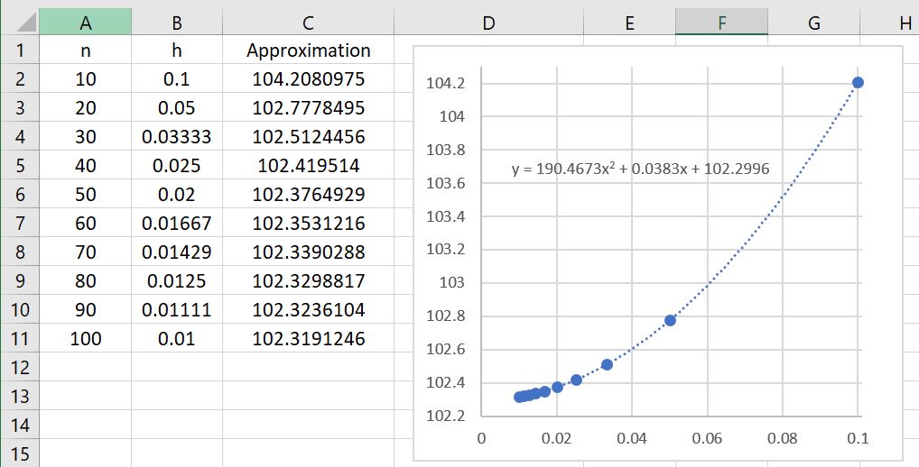
Once again, the data points fit a quadratic polynomial well, indicating quadratic convergence.
More subtly, it appears that the Trapezoid Rule isn’t quite as good as the Midpoint Rule. Here are the results from the Midpoint Rule (which also appeared in the previous post in this series):
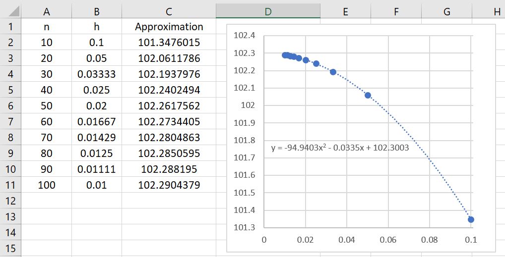
For 


To me, this is far from an obvious conclusion. Geometrically, it’s far from clear that the rectangles from the Midpoint Rule…

… provide a better approximation than using trapezoids …
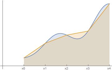
… yet it appears that’s exactly what happened. This can be rigorously proven, as we’ll explore later in this series.
 , using only ten subintervals, is a far better approximation than (from the previous post) either
  or
or  using 100 subintervals! The lesson to learn: choosing a good algorithm is often far better than simply doing lots of computations.
 and
and  subintervals. Geometrically, it’s clear that the orange rectangles in the second picture do a better job of approximating the area under the curve.

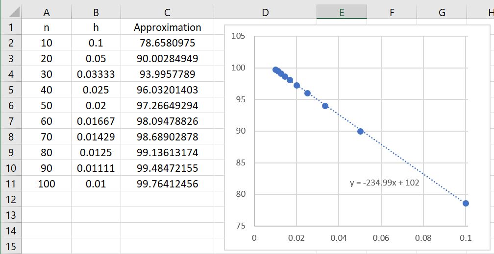
 are indeed getting closer and closer to the actual value of
  is plotted with these approximations, the data points fall almost exactly on a straight line. The same phenomenon occurs when using right endpoints:
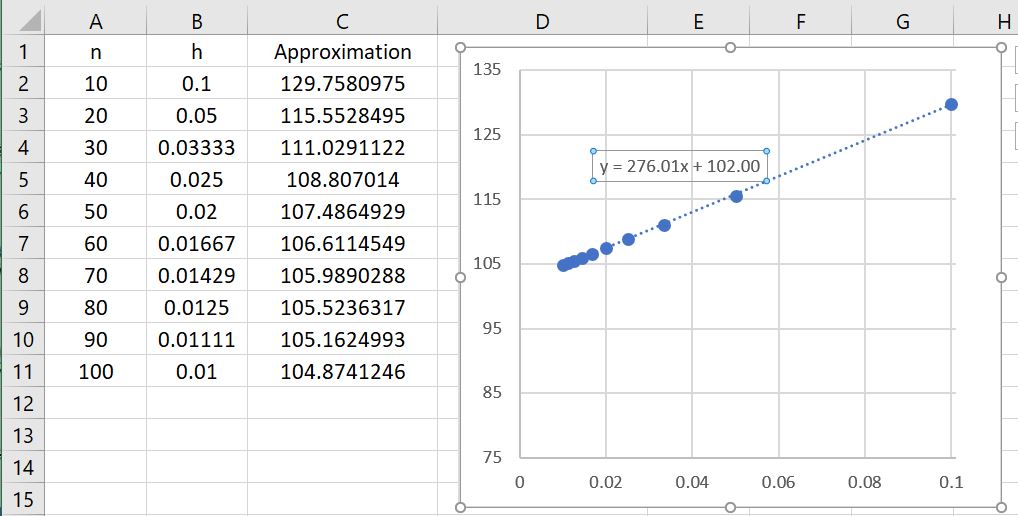
 using
using  subintervals, so that
 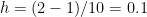 . To implement the left-endpoint rule, I enter the labels “x” and “x^9” in cells A1 and B1 of a spreadsheet. I then enter 1 (the left endpoint) in cell A2. In cell A3, I enter “=A2+0.1”, instructing the spreadsheet to add 0.1 to the value in cell A2. Then, instead of typing all of the other values of
  , I use the fill-down feature to repeat this pattern for cells A3 through A11. In cell B2, I enter “=A1^9”, applying the function
  to the
  coordinate in cell A2. Again, I use the fill-down feature to repeat this pattern for cells B3-B11. The fill-down feature saves a lot of time! Finally, in cell B13, I enter “=0.1*SUM(B2:B11)”, adding the values in cells B2 through B11 and multiplying the sum by
  , is the approximation using the left-endpoint rule with 10 subintervals.

![[1,1.01]](https://s0.wp.com/latex.php?latex=%5B1%2C1.01%5D&bg=ffffff&fg=000000&s=0&c=20201002) .
. 
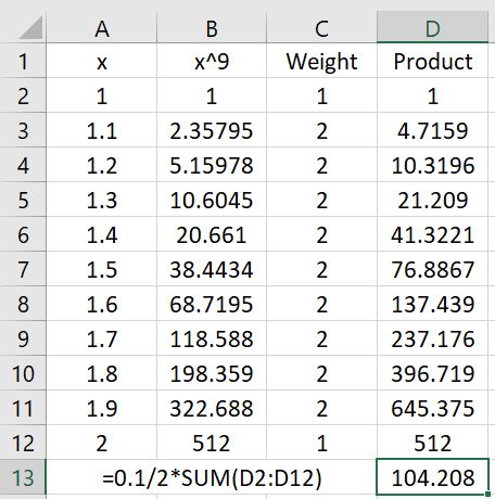
 . Again, these could be typed by hand, but it’s easiest to enter 4 in cell C3, 2 in cell C4, and then “=C3” in cell C5. The fill-down feature can take care of the rest of the weights. The Simpson’s Rule approximation is obtained by typing “=0.1/3*SUM(D2:D12)” in cell D13, with a new denominator of 3.
 subintervals with
  and
and  ,
,  ,
,  , and so on. Then Simpson’s Rule becomes
![S_{2n} = \displaystyle \frac{h}{3} \left[y_0 + 4 y_1 + 2 y_2 + 4 y_3 + \dots + 2y_{2n-2} + 4 y_{2n-1} + y_{2n} \right]](https://s0.wp.com/latex.php?latex=S_%7B2n%7D+%3D+%5Cdisplaystyle+%5Cfrac%7Bh%7D%7B3%7D+%5Cleft%5By_0+%2B+4+y_1+%2B+2+y_2+%2B+4+y_3+%2B+%5Cdots+%2B+2y_%7B2n-2%7D+%2B+4+y_%7B2n-1%7D+%2B%C2%A0+y_%7B2n%7D+%5Cright%5D&bg=ffffff&fg=000000&s=0&c=20201002) .
. , which is equal to
  . (In other words, since there are half as many subintervals, each one is twice as long.) Also, the endpoints of these subintervals will be
  , and so on. So, keeping the same labeling convention as with Simpson’s Rule, the Trapezoid Rule becomes
![T_n = \displaystyle \frac{2h}{2} [f(x_0) + 2f(x_2) + 2f(x_4) + \dots + 2f(x_{2n-2}) + f(x_{2n})]](https://s0.wp.com/latex.php?latex=T_n+%3D+%5Cdisplaystyle+%5Cfrac%7B2h%7D%7B2%7D+%5Bf%28x_0%29+%2B+2f%28x_2%29+%2B+2f%28x_4%29+%2B+%5Cdots+%2B+2f%28x_%7B2n-2%7D%29+%2B+f%28x_%7B2n%7D%29%5D&bg=ffffff&fg=000000&s=0&c=20201002)
![= h [f(x_0) + 2f(x_2) + 2f(x_4) + \dots + 2f(x_{2n-2}) + f(x_{2n})]](https://s0.wp.com/latex.php?latex=%3D+h+%5Bf%28x_0%29+%2B+2f%28x_2%29+%2B+2f%28x_4%29+%2B+%5Cdots+%2B+2f%28x_%7B2n-2%7D%29+%2B+f%28x_%7B2n%7D%29%5D&bg=ffffff&fg=000000&s=0&c=20201002) .
. .) Furthermore, the midpoint of subinterval
 ![[x_0, x_2]](https://s0.wp.com/latex.php?latex=%5Bx_0%2C+x_2%5D&bg=ffffff&fg=000000&s=0&c=20201002) will be
will be  , the midpoint of subinterval
 ![[x_2,x_4]](https://s0.wp.com/latex.php?latex=%5Bx_2%2Cx_4%5D&bg=ffffff&fg=000000&s=0&c=20201002) will be
will be  , and so on. Therefore, keeping the same labeling convention, the Midpoint Rule becomes
![M_n = \displaystyle 2h [f(x_1) + f(x_3) + f(x_5) + \dots + f(x_{2n-1}) ]](https://s0.wp.com/latex.php?latex=M_n+%3D+%5Cdisplaystyle+2h+%5Bf%28x_1%29+%2B+f%28x_3%29+%2B+f%28x_5%29+%2B+%5Cdots+%2B+f%28x_%7B2n-1%7D%29+%5D&bg=ffffff&fg=000000&s=0&c=20201002) .
. , a certain weighted average of
  and
and  , is equal to
![\displaystyle \frac{4h}{3} [f(x_1) + f(x_3) + \dots + f(x_{2n-1}) ] + \frac{h}{3} [f(x_0) + 2f(x_2) + \dots + 2f(x_{2n-2}) + f(x_{2n})]](https://s0.wp.com/latex.php?latex=%5Cdisplaystyle+%5Cfrac%7B4h%7D%7B3%7D+%5Bf%28x_1%29+%2B+f%28x_3%29+%2B+%5Cdots+%2B+f%28x_%7B2n-1%7D%29+%5D+%2B+%5Cfrac%7Bh%7D%7B3%7D+%5Bf%28x_0%29+%2B+2f%28x_2%29+%2B+%5Cdots+%2B+2f%28x_%7B2n-2%7D%29+%2B+f%28x_%7B2n%7D%29%5D&bg=ffffff&fg=000000&s=0&c=20201002)
![= \displaystyle \frac{h}{3} [f(x_0) + 4 f(x_1) + 2f(x_2) + \dots + 2f(x_{2n-2}) + 4 f(x_{2n-1} + f(x_{2n})]](https://s0.wp.com/latex.php?latex=%3D+%5Cdisplaystyle%C2%A0+%5Cfrac%7Bh%7D%7B3%7D+%5Bf%28x_0%29+%2B+4+f%28x_1%29+%2B+2f%28x_2%29+%2B+%5Cdots+%2B+2f%28x_%7B2n-2%7D%29+%2B+4+f%28x_%7B2n-1%7D+%2B+f%28x_%7B2n%7D%29%5D&bg=ffffff&fg=000000&s=0&c=20201002)
 .
. and
and  , and so the area of the first trapezoid is
 ![\frac{1}{2} h[ f(x_0) + f(x_1) ]](https://s0.wp.com/latex.php?latex=%5Cfrac%7B1%7D%7B2%7D+h%5B+f%28x_0%29+%2B+f%28x_1%29+%5D&bg=ffffff&fg=000000&s=0&c=20201002) . The other areas are found similarly. Adding these together, we get the approximation
. The other areas are found similarly. Adding these together, we get the approximation![T_n = \displaystyle \frac{h}{2}[f(x_0) + f(x_1)] + \frac{h}{2} [f(x_1) + f(x_2)] + \dots +](https://s0.wp.com/latex.php?latex=T_n+%3D+%5Cdisplaystyle+%5Cfrac%7Bh%7D%7B2%7D%5Bf%28x_0%29+%2B+f%28x_1%29%5D+%2B+%5Cfrac%7Bh%7D%7B2%7D+%5Bf%28x_1%29+%2B+f%28x_2%29%5D+%2B+%5Cdots+%2B+&bg=ffffff&fg=000000&s=0&c=20201002)
![+ \displaystyle \frac{h}{2} [f(x_{n-2})+f(x_{n-1})] + \frac{h}{2} [f(x_{n-1})+f(x_n)]](https://s0.wp.com/latex.php?latex=%2B+%5Cdisplaystyle+%5Cfrac%7Bh%7D%7B2%7D+%5Bf%28x_%7Bn-2%7D%29%2Bf%28x_%7Bn-1%7D%29%5D+%2B+%5Cfrac%7Bh%7D%7B2%7D+%5Bf%28x_%7Bn-1%7D%29%2Bf%28x_n%29%5D&bg=ffffff&fg=000000&s=0&c=20201002)
![= \displaystyle \frac{h}{2} [f(x_0) + 2f(x_1) + 2f(x_2) + \dots + 2f(x_{n-2}) + 2f(x_{n-1}) + f(x_n)].](https://s0.wp.com/latex.php?latex=%3D+%5Cdisplaystyle+%5Cfrac%7Bh%7D%7B2%7D+%5Bf%28x_0%29+%2B+2f%28x_1%29+%2B+2f%28x_2%29+%2B+%5Cdots+%2B+2f%28x_%7Bn-2%7D%29+%2B+2f%28x_%7Bn-1%7D%29+%2B+f%28x_n%29%5D.&bg=ffffff&fg=000000&s=0&c=20201002)
 :
:
![= \displaystyle \frac{h}{2} \left[f(x_0) + f(x_1) + f(x_2) + \dots + f(x_{n-1}) \right]](https://s0.wp.com/latex.php?latex=%3D+%5Cdisplaystyle+%5Cfrac%7Bh%7D%7B2%7D+%5Cleft%5Bf%28x_0%29+%2B+f%28x_1%29+%2B+f%28x_2%29+%2B+%5Cdots+%2B+f%28x_%7Bn-1%7D%29+%5Cright%5D&bg=ffffff&fg=000000&s=0&c=20201002)
![+\displaystyle \frac{h}{2} \left[f(x_1) + f(x_2) + \dots + f(x_{n-1}) + f(x_{n}) \right]](https://s0.wp.com/latex.php?latex=%2B%5Cdisplaystyle+%5Cfrac%7Bh%7D%7B2%7D+%5Cleft%5Bf%28x_1%29+%2B+f%28x_2%29+%2B+%5Cdots+%2B+f%28x_%7Bn-1%7D%29+%2B+f%28x_%7Bn%7D%29+%5Cright%5D&bg=ffffff&fg=000000&s=0&c=20201002)
![= \displaystyle \frac{h}{2} \left[f(x_0) + 2f(x_1) + \dots + 2f(x_{n-1}) + f(x_n) \right]](https://s0.wp.com/latex.php?latex=%3D+%5Cdisplaystyle+%5Cfrac%7Bh%7D%7B2%7D+%5Cleft%5Bf%28x_0%29+%2B+2f%28x_1%29+%2B+%5Cdots+%2B+2f%28x_%7Bn-1%7D%29+%2B+f%28x_n%29+%5Cright%5D&bg=ffffff&fg=000000&s=0&c=20201002)
 .
. , so that
  ,
,  , and
, and  . We then can draw rectangles using the left endpoints of each subinterval. The sum of the areas of these rectangles below is
 ,
,![\int_a^b f(x) \, dx \approx h \left[f(x_0) + f(x_1) + \dots + f(x_{n-1}) \right]](https://s0.wp.com/latex.php?latex=%5Cint_a%5Eb+f%28x%29+%5C%2C+dx+%5Capprox+h+%5Cleft%5Bf%28x_0%29+%2B+f%28x_1%29+%2B+%5Cdots+%2B+f%28x_%7Bn-1%7D%29+%5Cright%5D&bg=ffffff&fg=000000&s=0&c=20201002)
 ,
,![\int_a^b f(x) \, dx \approx h \left[f(x_1) + f(x_2) + \dots + f(x_n) \right]](https://s0.wp.com/latex.php?latex=%5Cint_a%5Eb+f%28x%29+%5C%2C+dx+%5Capprox+h+%5Cleft%5Bf%28x_1%29+%2B+f%28x_2%29+%2B+%5Cdots+%2B+f%28x_n%29+%5Cright%5D&bg=ffffff&fg=000000&s=0&c=20201002)

 . The sum of the areas of the rectangles below is
 ,
,![\int_a^b f(x) \, dx \approx h \left[f(c_1) + f(c_2) + \dots + f(c_n) \right]](https://s0.wp.com/latex.php?latex=%5Cint_a%5Eb+f%28x%29+%5C%2C+dx+%5Capprox+h+%5Cleft%5Bf%28c_1%29+%2B+f%28c_2%29+%2B+%5Cdots+%2B+f%28c_n%29+%5Cright%5D&bg=ffffff&fg=000000&s=0&c=20201002)
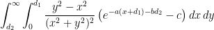
 , which is closely related to the area under the bell curve
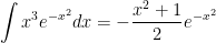
  . This integral cannot be computed using elementary functions. However, using integration by parts, there are some related integrals that can be computed:


 ,
, , a polynomial of degree
 ![\displaystyle \frac{d}{dx} \left[ f(x) e^{-x^2} \right] = e^{-x^2}](https://s0.wp.com/latex.php?latex=%5Cdisplaystyle+%5Cfrac%7Bd%7D%7Bdx%7D+%5Cleft%5B+f%28x%29+e%5E%7B-x%5E2%7D+%5Cright%5D+%3D+e%5E%7B-x%5E2%7D&bg=ffffff&fg=000000&s=0&c=20201002)

 .
. is a polynomial of degree
  while
while  is a polynomial of degree
  . Therefore, the left hand side must have degree
  , where the exponents
  may or may not be integers.
  . Indeed, although the proof goes well beyond first-year calculus, there is a theorem that says that if
  can be expressed in terms of elementary functions, then the antiderivative must have the form
  . So the guess above actually can be rigorously justified. References:
 to find
  .
. to find

 , otherwise known as the bell curve. For most numbers
  and
and  , the area


![\displaystyle \int_0^{2R} e^{-sz} \exp \left[ -c \left( z \sqrt{4R^2-z^2} + 4R^2 \arcsin \frac{z}{2R} \right) \right] dz](https://s0.wp.com/latex.php?latex=%5Cdisplaystyle+%5Cint_0%5E%7B2R%7D+e%5E%7B-sz%7D+%5Cexp+%5Cleft%5B+-c+%5Cleft%28+z+%5Csqrt%7B4R%5E2-z%5E2%7D%C2%A0+%2B+4R%5E2+%5Carcsin+%5Cfrac%7Bz%7D%7B2R%7D+%5Cright%29+%5Cright%5D+dz&bg=ffffff&fg=000000&s=0&c=20201002)
![\displaystyle \int_0^d \exp \left[ -sz - \lambda \left(z - \frac{z^2}{4d} \right) \right] dz](https://s0.wp.com/latex.php?latex=%5Cdisplaystyle+%5Cint_0%5Ed+%5Cexp+%5Cleft%5B+-sz+-+%5Clambda+%5Cleft%28z+-+%5Cfrac%7Bz%5E2%7D%7B4d%7D+%5Cright%29+%5Cright%5D+dz&bg=ffffff&fg=000000&s=0&c=20201002)
![\displaystyle \int_d^{d \sqrt{2}} \exp \left[ -sz - \lambda \left( \frac{d (\pi+1)}{2} - d \arcsin \frac{d}{z} + \frac{z^2}{4d} - \sqrt{z^2-d^2} \right) \right] dz](https://s0.wp.com/latex.php?latex=%5Cdisplaystyle+%5Cint_d%5E%7Bd+%5Csqrt%7B2%7D%7D+%5Cexp+%5Cleft%5B+-sz+-+%5Clambda+%5Cleft%28+%5Cfrac%7Bd+%28%5Cpi%2B1%29%7D%7B2%7D+-+d+%5Carcsin+%5Cfrac%7Bd%7D%7Bz%7D+%2B+%5Cfrac%7Bz%5E2%7D%7B4d%7D+-+%5Csqrt%7Bz%5E2-d%5E2%7D+%5Cright%29+%5Cright%5D+dz&bg=ffffff&fg=000000&s=0&c=20201002)
![\displaystyle \int_0^\infty \exp \left[-sz - \eta \left(1 - e^{-cz/2} - \frac{cz}{4} e^{-cz/2} \right) \right] dz](https://s0.wp.com/latex.php?latex=%5Cdisplaystyle+%5Cint_0%5E%5Cinfty+%5Cexp+%5Cleft%5B-sz+-+%5Ceta+%5Cleft%281+-+e%5E%7B-cz%2F2%7D+-+%5Cfrac%7Bcz%7D%7B4%7D+e%5E%7B-cz%2F2%7D+%5Cright%29+%5Cright%5D+dz&bg=ffffff&fg=000000&s=0&c=20201002)