Peer-reviewed publications is the best way that we’ve figured out for vetting scientific experiments and disseminating scientific knowledge. But that doesn’t mean that the system can’t be abused, either consciously or unconsciously.

The eye-opening article http://io9.com/i-fooled-millions-into-thinking-chocolate-helps-weight-1707251800 describes how the author published flimsy data that any discerning statistician should have seen through and even managed to get his “results” spread in the popular press. Some money quotes:

Here’s a dirty little science secret: If you measure a large number of things about a small number of people, you are almost guaranteed to get a “statistically significant” result. Our study included 18 different measurements—weight, cholesterol, sodium, blood protein levels, sleep quality, well-being, etc.—from 15 people. (One subject was dropped.) That study design is a recipe for false positives.

Think of the measurements as lottery tickets. Each one has a small chance of paying off in the form of a “significant” result that we can spin a story around and sell to the media. The more tickets you buy, the more likely you are to win. We didn’t know exactly what would pan out—the headline could have been that chocolate improves sleep or lowers blood pressure—but we knew our chances of getting at least one “statistically significant” result were pretty good.

And:

With the paper out, it was time to make some noise. I called a friend of a friend who works in scientific PR. She walked me through some of the dirty tricks for grabbing headlines. It was eerie to hear the other side of something I experience every day.

The key is to exploit journalists’ incredible laziness. If you lay out the information just right, you can shape the story that emerges in the media almost like you were writing those stories yourself. In fact, that’s literally what you’re doing, since many reporters just copied and pasted our text.

And:

The only problem with the diet science beat is that it’s science. You have to know how to read a scientific paper—and actually bother to do it. For far too long, the people who cover this beat have treated it like gossip, echoing whatever they find in press releases. Hopefully our little experiment will make reporters and readers alike more skeptical.

If a study doesn’t even list how many people took part in it, or makes a bold diet claim that’s “statistically significant” but doesn’t say how big the effect size is, you should wonder why. But for the most part, we don’t. Which is a pity, because journalists are becoming the de facto peer review system. And when we fail, the world is awash in junk science.

The Extent and Consequences of P-Hacking in Science

A couple months ago, the open-access journal PLOS Biology (which is a reputable open-access journal, unlike many others) published this very interesting article about the abuse of hypothesis testing in the scientific literature: http://journals.plos.org/plosbiology/article?id=10.1371%2Fjournal.pbio.1002106

Here are some of my favorite quotes from near the end of the article:

The key to decreasing p-hacking is better education of researchers. Many practices that lead to p-hacking are still deemed acceptable. John et al. measured the prevalence of questionable research practices in psychology. They asked survey participants if they had ever engaged in a set of questionable research practices and, if so, whether they thought their actions were defensible on a scale of 0–2 (0 = no, 1 = possibly, 2 = yes). Over 50% of participants admitted to “failing to report all of a study’s dependent measures” and “deciding whether to collect more data after looking to see whether the results were significant,” and these practices received a mean defensibility rating greater than 1.5. This indicates that many researchers p-hack but do not appreciate the extent to which this is a form of scientific misconduct. Amazingly, some animal ethics boards even encourage or mandate the termination of research if a significant result is obtained during the study, which is a particularly egregious form of p-hacking (Anonymous reviewer, personal communication).

Eliminating p-hacking entirely is unlikely when career advancement is assessed by publication output, and publication decisions are affected by the p-value or other measures of statistical support for relationships. Even so, there are a number of steps that the research community and scientific publishers can take to decrease the occurrence of p-hacking.

Student t distribution

One of my favorite anecdotes that I share with my statistics students is why the Student t distribution is called the t distribution and not the Gosset distribution.

From Wikipedia:

In the English-language literature it takes its name from William Sealy Gosset’s 1908 paper in Biometrika under the pseudonym “Student”. Gosset worked at the Guinness Brewery in Dublin, Ireland, and was interested in the problems of small samples, for example the chemical properties of barley where sample sizes might be as low as 3. One version of the origin of the pseudonym is that Gosset’s employer preferred staff to use pen names when publishing scientific papers instead of their real name, therefore he used the name “Student” to hide his identity. Another version is that Guinness did not want their competitors to know that they were using the t-test to test the quality of raw material.

Gosset’s paper refers to the distribution as the “frequency distribution of standard deviations of samples drawn from a normal population”. It became well-known through the work of Ronald A. Fisher, who called the distribution “Student’s distribution” and referred to the value as t.

From the 1963 book Experimentation and Measurement (see pages 68-69 of the PDF, which are marked as pages 69-70 on the original):

The mathematical solution to this problem was first discovered by an Irish chemist who wrote under the pen name of “Student.” Student worked for a company that was unwilling to reveal its connection with him lest its competitors discover that Student’s work would also be advantageous to them. It now seems extraordinary that the author of this classic paper on measurements was not known for more than twenty years. Eventually it was learned that his real name was William Sealy Gosset (1876-1937).

A T-shirt describing hypothesis testing

Mathematical Christmas gifts

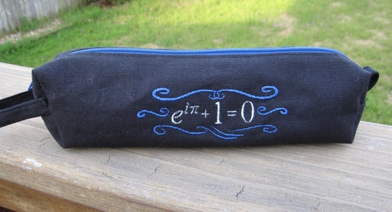
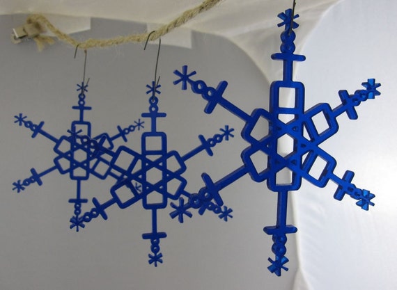
Now that Christmas is over, I can safely share the Christmas gifts that I gave to my family this year thanks to Nausicaa Distribution (https://www.etsy.com/shop/NausicaaDistribution):

Euler’s equation pencil pouch:

Box-and-whisker snowflakes to hang on our Christmas tree:

And, for me, a wonderfully and subtly punny “Confidence and Power” T-shirt.

Thanks to FiveThirtyEight (see http://fivethirtyeight.com/features/the-fivethirtyeight-2014-holiday-gift-guide/) for pointing me in this direction.

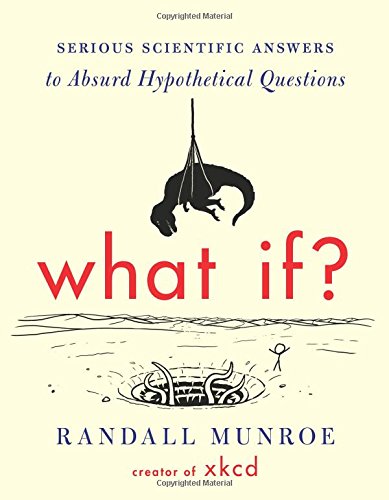
For the sake of completeness, here are the math-oriented gifts that I received for Christmas:

Null hypothesis

Source: http://xkcd.com/892/

Rejection regions

Sage words of wisdom that I gave one day in my statistics class:

If the alternative hypothesis has the form $p > p_0$ , then the rejection region lies to the right of $p_0$ . On the other hand, if the alternative hypothesis has the form $p < p_0$ , then the rejection region lies to the left of $p_0$ .

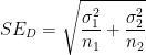
On the other hand, if the alternative hypothesis has the form $p \ne p_0$ , then the rejection region has two parts: one part to the left of $p_0$ , and another part to the right. So it’s kind of like my single days. Back then, my rejection region had two parts: Friday night and Saturday night.

Welch’s formula

When conducting an hypothesis test or computing a confidence interval for the difference $\overline{X}_1 - \overline{X}_2$ of two means, where at least one mean does not arise from a small sample, the Student t distribution must be employed. In particular, the number of degrees of freedom for the Student t distribution must be computed. Many textbooks suggest using Welch’s formula:

$df = \frac{\displaystyle (SE_1^2 + SE_2^2)^2}{\displaystyle \frac{SE_1^4}{n_1-1} + \frac{SE_2^4}{n_2-1}},$

rounded down to the nearest integer. In this formula, $SE_1 = \displaystyle \frac{\sigma_1}{\sqrt{n_1}}$ is the standard error associated with the first average $\overline{X}_1$ , where $\sigma_1$ (if known) is the population standard deviation for $X$ and $n_1$ is the number of samples that are averaged to find $\overline{X}_1$ . In practice, $\sigma_1$ is not known, and so the bootstrap estimate $\sigma_1 \approx s_1$ is employed.

The terms $SE_2$ and $n_2$ are similarly defined for the average $\overline{X}_2$ .

In Welch’s formula, the term $SE_1^2 + SE_2^2$ in the numerator is equal to $\displaystyle \frac{\sigma_1^2}{n_1} + \frac{\sigma_2^2}{n_2}$ . This is the square of the standard error $SE_D$ associated with the difference $\overline{X}_1 - \overline{X}_2$ , since

$SE_D = \displaystyle \sqrt{\frac{\sigma_1^2}{n_1} + \frac{\sigma_2^2}{n_2}}$ .

This leads to the “Pythagorean” relationship

$SE_1^2 + SE_2^2 = SE_D^2$ ,

which (in my experience) is a reasonable aid to help students remember the formula for $SE_D$ .

Naturally, a big problem that students encounter when using Welch’s formula is that the formula is really, really complicated, and it’s easy to make a mistake when entering information into their calculators. (Indeed, it might be that the pre-programmed calculator function simply gives the wrong answer.) Also, since the formula is complicated, students don’t have a lot of psychological reassurance that, when they come out the other end, their answer is actually correct. So, when teaching this topic, I tell my students the following rule of thumb so that they can at least check if their final answer is plausible:

$\min(n_1,n_2)-1 \le df \le n_1 + n_2 -2$ .

To my surprise, I have never seen this formula in a statistics textbook, even though it’s quite simple to state and not too difficult to prove using techniques from first-semester calculus.

Let’s rewrite Welch’s formula as

$df = \left( \displaystyle \frac{1}{n_1-1} \left[ \frac{SE_1^2}{SE_1^2 + SE_2^2}\right]^2 + \frac{1}{n_2-1} \left[ \frac{SE_2^2}{SE_1^2 + SE_2^2} \right]^2 \right)^{-1}$

For the sake of simplicity, let $m_1 = n_1 - 1$ and $m_2 = n_2 -1$ , so that

$df = \left( \displaystyle \frac{1}{m_1} \left[ \frac{SE_1^2}{SE_1^2 + SE_2^2}\right]^2 + \frac{1}{m_2} \left[ \frac{SE_2^2}{SE_1^2 + SE_2^2} \right]^2 \right)^{-1}$

Now let $x = \displaystyle \frac{SE_1^2}{SE_1^2 + SE_2^2}$ . All of these terms are nonnegative (and, in practice, they’re all positive), so that $x \ge 0$ . Also, the numerator is no larger than the denominator, so that $x \le 1$ . Finally, we notice that

$1-x = 1 - \displaystyle \frac{SE_1^2}{SE_1^2 + SE_2^2} = \frac{SE_2^2}{SE_1^2 + SE_2^2}$ .

Using these observations, Welch’s formula reduces to the function

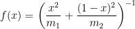
$f(x) = \left( \displaystyle \frac{x^2}{m_1} + \frac{(1-x)^2}{m_2} \right)^{-1}$ ,

and the central problem is to find the maximum and minimum values of $f(x)$ on the interval $0 \le x \le 1$ . Since $f(x)$ is differentiable on $[0,1]$ , the absolute extrema can be found by checking the endpoints and the critical point(s).

First, the endpoints. If $x=0$ , then $f(0) = \left( \displaystyle \frac{1}{m_2} \right)^{-1} = m_2$ . On the other hand, if $x=1$ , then $f(1) = \left( \displaystyle \frac{1}{m_1} \right)^{-1} = m_1$ .

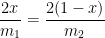
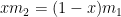
Next, the critical point(s). These are found by solving the equation $f'(x) = 0$ :

$f'(x) = -\left( \displaystyle \frac{x^2}{m_1} + \frac{(1-x)^2}{m_2} \right)^{-2} \left[ \displaystyle \frac{2x}{m_1} - \frac{2(1-x)}{m_2} \right] = 0$

$\displaystyle \frac{2x}{m_1} - \frac{2(1-x)}{m_2} = 0$

$\displaystyle \frac{2x}{m_1} = \frac{2(1-x)}{m_2}$

$xm_2= (1-x)m_1$

$xm_2 = m_1 - xm_1$

$x(m_1 + m_2) = m_1$

$x = \displaystyle \frac{m_1}{m_1 + m_2}$

Plugging back into the original equation, we find the local extremum

$f \left( \displaystyle \frac{m_1}{m_1+m_2} \right) = \left( \displaystyle \frac{1}{m_1} \frac{m_1^2}{(m_1+m_2)^2} + \frac{1}{m_2} \left[1-\frac{m_1}{m_1+m_2}\right]^2 \right)^{-1}$

$f \left( \displaystyle \frac{m_1}{m_1+m_2} \right) = \left( \displaystyle \frac{1}{m_1} \frac{m_1^2}{(m_1+m_2)^2} + \frac{1}{m_2} \left[\frac{m_2}{m_1+m_2}\right]^2 \right)^{-1}$

$f \left( \displaystyle \frac{m_1}{m_1+m_2} \right) = \left( \displaystyle \frac{m_1}{(m_1+m_2)^2} + \frac{m_2}{(m_1+m_2)^2} \right)^{-1}$

$f \left( \displaystyle \frac{m_1}{m_1+m_2} \right) = \left( \displaystyle \frac{m_1+m_2}{(m_1+m_2)^2} \right)^{-1}$

$f \left( \displaystyle \frac{m_1}{m_1+m_2} \right) = \left( \displaystyle \frac{1}{m_1+m_2} \right)^{-1}$

$f \left( \displaystyle \frac{m_1}{m_1+m_2} \right) = m_1+m_2$

Based on the three local extrema that we’ve found, it’s clear that the absolute minimum of $f(x)$ on $[0,1]$ is the smaller of $m_1$ and $m_2$ , while the absolute maximum is equal to $m_1 + m_2$ .

$\hbox{QED}$

In conclusion, I suggest offering the following guidelines to students to encourage their intuition about the plausibility of their answers:

If $SE_1$ is much smaller than $SE_2$ (i.e., $x \approx 0$ ), then $df$ will be close to $m_2 = n_2 - 1$ .
If $SE_1$ is much larger than $SE_2$ (i.e., $x \approx 1$ ), then $df$ will be close to $m_1 = n_1 - 1$ .
Otherwise, $df$ could be as large as $m_1 + m_2 = n_1 + n_2 - 2$ , but no larger.

Statistical significance

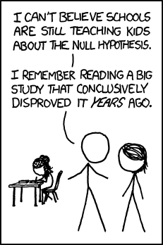
When teaching my Applied Statistics class, I’ll often use the following xkcd comic to reinforce the meaning of statistical significance.

The idea that’s being communicated is that, when performing an hypothesis test, the observed significance level $P$ is the probability that the null hypothesis is correct due to dumb luck as opposed to a real effect (the alternative hypothesis). So if the significance level is really about $0.05$ and the experiment is repeated about 20 times, it wouldn’t be surprising for one of those experiments to falsely reject the null hypothesis.

In practice, statisticians use the Bonferroni correction when performing multiple simultaneous tests to avoid the erroneous conclusion displayed in the comic.

Source: http://www.xkcd.com/882/

Tag: hypothesis test

Interpreting statistical significance

io9: “I Fooled Millions Into Thinking Chocolate Helps Weight Loss. Here’s How.”